Optimization Techniques
Optimization Techniques in Machine Learning
Why Optimization?
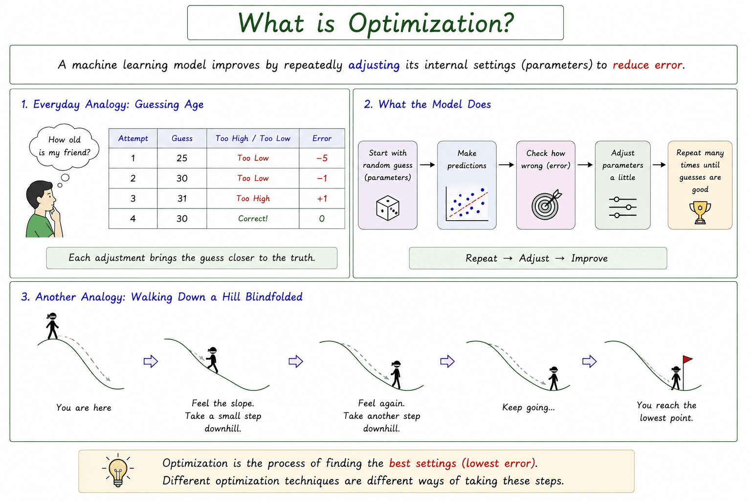
Imagine you're trying to guess a friend's age just by looking at them. Your first guess is probably wrong. So you adjust "okay, maybe a bit older" and guess again. And again. Each time, you get a little closer to the truth.
That's basically what a machine learning model does while it's "learning." It starts with a random guess for its internal settings (called parameters), checks how wrong that guess is, and then adjusts the settings to be a little less wrong. It repeats this thousands or millions of times until the guesses are good.
Optimization is just the name for this "adjust and improve" process. It's the set of rules that tell the model exactly how to change its settings after each wrong guess, so that it gets better instead of worse or random.
A nice way to picture it: you're standing somewhere on a hilly landscape, blindfolded, and your goal is to reach the lowest point in the valley. You can't see anything, but you can feel which way the ground slopes under your feet. So you take a small step downhill, feel the slope again, take another step, and so on until you can't go any lower. That's optimization in a nutshell, and the rest of this chapter is just different strategies for taking those steps well.
Residual & Error
Before you can improve a guess, you need a way to measure how wrong it is.
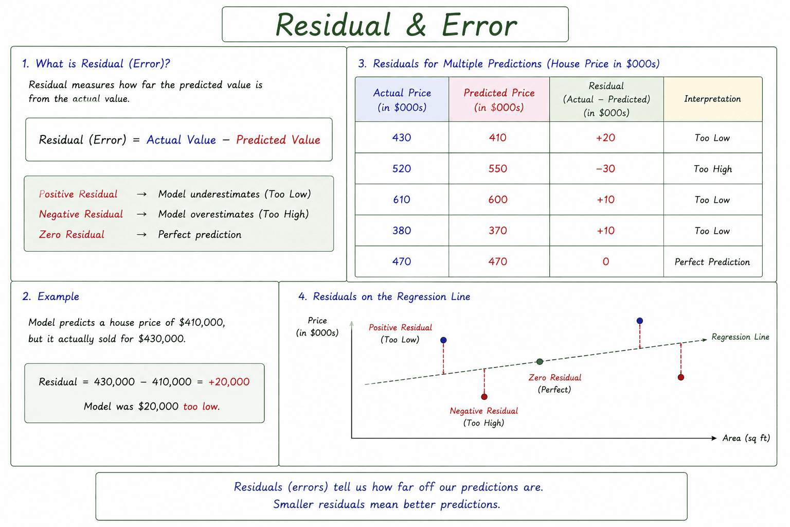
The simplest measurement is the residual: just the actual answer minus the model's guess.
\[residual = actual value − predicted value\]
Say a model predicts a house will sell for $410,000, but it actually sold for $430,000. The residual is $20,000 the model was $20,000 too low. Do this for every prediction the model makes, and you get a residual for each one. People also just call this the "error," and for our purposes the two words mean the same thing.
Loss Function vs Cost Function
Now you have a pile of individual errors (residuals) one per prediction. But to actually improve the model, you need a single number that sums up "how well is the model doing overall?"
This is where two easily-confused terms come in:
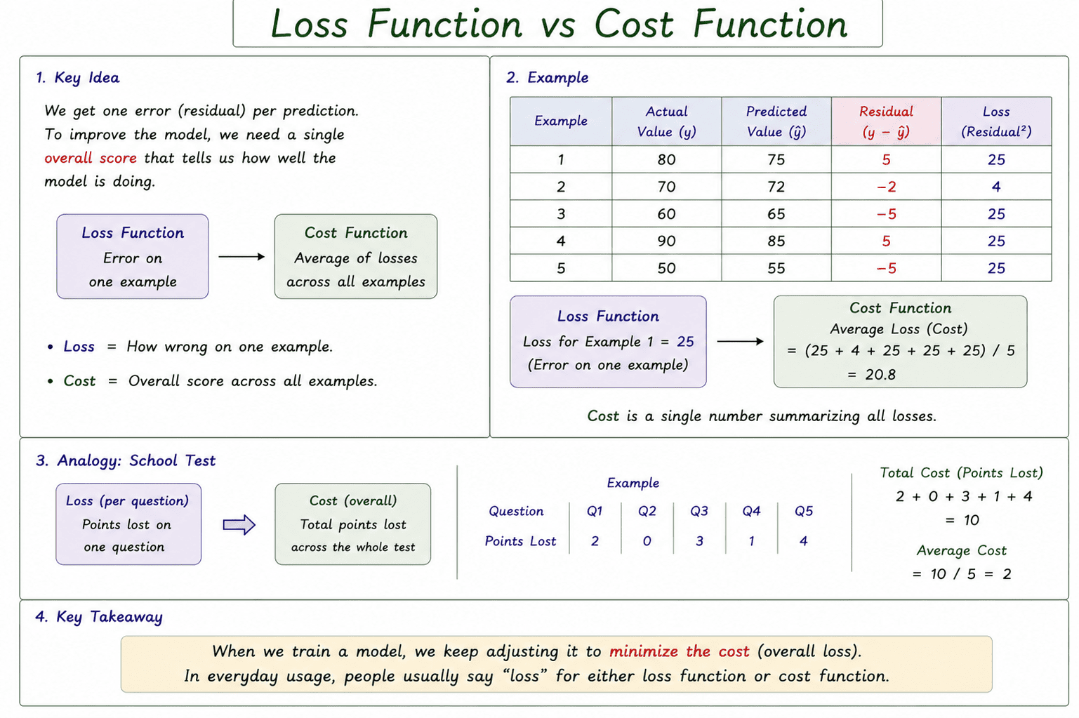
- A loss function tells you how wrong the model was on one single example.
- A cost function takes the loss from every example and averages them into one overall score.
Think of it like a test at school: the loss is how many points you lost on one question, and the cost is your final score across the whole test. When people talk about "training" a model, what they really mean is: keep adjusting the model until this overall score (the cost) gets as low as possible.
In casual conversation (and in most tutorials, including this one from here on) people just say "loss" to mean either one it's usually clear from context.
Common Loss/Cost Functions
There's more than one way to measure "wrongness," and the one you pick changes how the model behaves. Here are the four you'll run into constantly.
MSE / RMSE
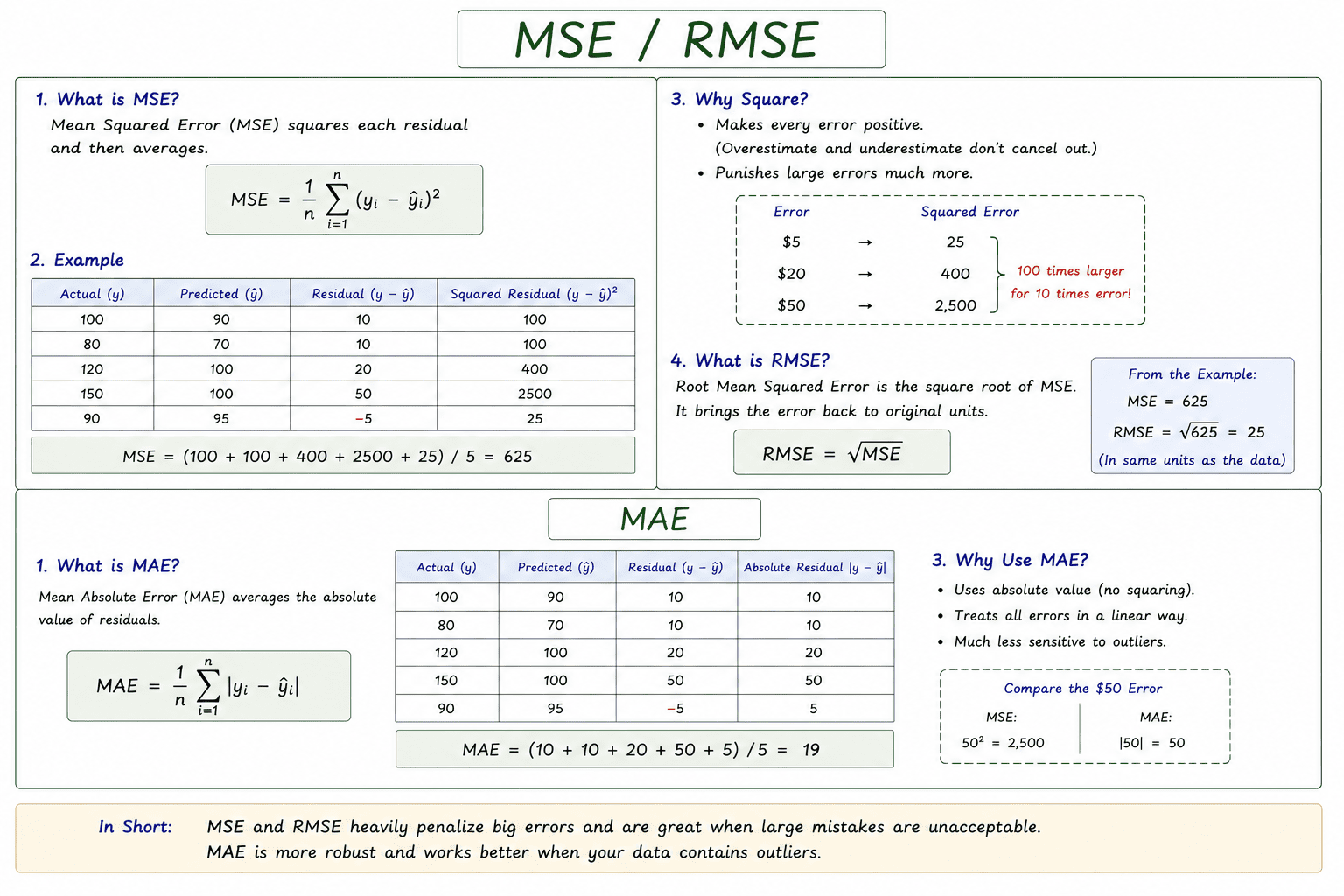
Mean Squared Error (MSE) takes every residual, squares it (multiplies it by itself), and then averages all those squared numbers.
Why square it? Two reasons. First, squaring turns every error positive, so a $20 overestimate and a $20 underestimate don't cancel each other out. Second, squaring punishes big mistakes much more than small ones. A $5 error becomes 25. A $50 error becomes 2,500, 100 times worse, not 10 times worse.
This makes MSE great at pushing the model to avoid large mistakes, but it also means one huge outlier can throw the whole score off.
For example, if four predictions are off by $5 but one prediction is off by $50, the $50 error contributes 2,500 to the MSE, while each $5 error contributes only 25. As a result, that one large mistake can dominate the overall MSE, even if the other predictions are quite accurate.
Root Mean Squared Error (RMSE) is just the square root of MSE. It exists purely so the number makes sense again in normal units. MSE on house prices is measured in dollars squared (dollars²), which doesn't mean much to anyone. Taking the square root converts it back to plain dollars. So, if your RMSE is $15,000, you can simply say that the model's predictions are typically off by about $15,000. That's why RMSE is often preferred when explaining a model's performance to non-technical people—it is much easier to understand than MSE.
MAE
Mean Absolute Error (MAE) also averages the errors, but instead of squaring them, it just takes their absolute value (ignoring the +/− sign).
This makes MAE much gentler toward outliers than MSE a $50 error just counts as 50, not 2,500. If your data has a few weird, extreme values you don't want to dominate the results, MAE is usually the safer choice.
Interestingly, the measures discussed above have a dual role. During training, they are used as loss (or cost) functions that the model tries to minimize. After training, the same measures such as MSE, RMSE, and MAE are commonly used as performance metrics to evaluate the model's prediction accuracy.
Log Loss (Cross-Entropy)
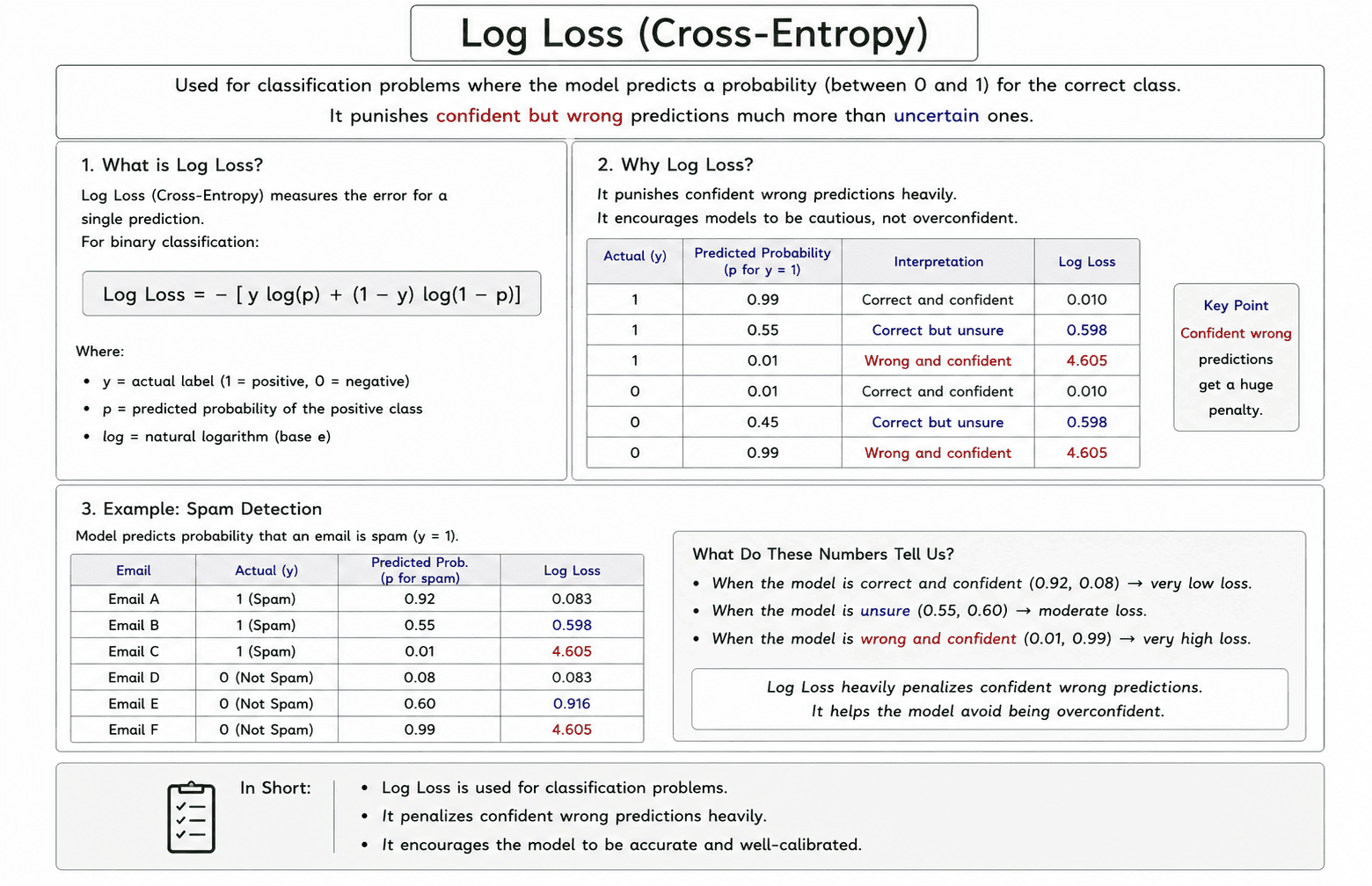
MSE and MAE work well when you're predicting a number—a price, a temperature, or a score. But many machine learning problems involve predicting a category instead, such as "Is this email spam or not spam?" In these cases, the model predicts a probability (for example, "92% sure this is spam"), so a different loss function called Log Loss (or Cross-Entropy Loss) is used.
The key idea behind log loss is that it punishes the model heavily when it is confidently wrong. If the model says, "I'm 99% sure this is not spam," but the email actually is spam, log loss gives a very large penalty. On the other hand, if the model says, "I'm only 55% sure this is not spam," and the email still turns out to be spam, the penalty is much smaller because the model admitted it was uncertain.
For example, consider two spam filters that both make the wrong prediction on the same email:
- Model A: "This email is 99% not spam." (Very confident, but wrong)
- Model B: "This email is 55% not spam." (Slightly confident, but wrong)
Both models are incorrect, but Model A receives a much larger log loss because it was extremely confident in its wrong prediction. Model B also loses points, but not nearly as many because it acknowledged some uncertainty.
This encourages the model to be confident only when it has strong evidence. Over time, the model learns not just to make correct predictions, but also to assign probabilities that accurately reflect its confidence.
A loss (or cost) function tells the model how wrong its predictions are. An optimization algorithm, such as OLS or Gradient Descent, uses that loss function to adjust the model's parameters until the loss becomes as small as possible.
Solving the Optimization Problem
So you've picked a way to measure wrongness (a loss/cost function). Now, how do you actually find the model settings that make that number as small as possible?
OLS
Ordinary Least Squares (OLS) is the classical analytical optimization technique used to train Linear Regression models. It computes the optimal model parameters (such as m and c in Simple Linear Regression) that produce the Best-Fit Line by minimizing the Sum of Squared Errors (SSE). Unlike iterative optimization methods, OLS directly calculates the optimal parameter values using mathematical formulas, without requiring repeated updates or guessing.
How OLS Works
The OLS method follows these steps:
- Collect the training dataset containing input (x) and output (y) values.
- Calculate the required summations:
\[∑x, ∑y, ∑x2, ∑xy∑xy\]
- Use the OLS formulas to compute the model parameters:
- Slope (m)
- Intercept (c)
- Construct the Best-Fit Line using the equation:
\[y=mx+c\]
Use the equation to predict new values and evaluate the model using residuals and error metrics.
OLS Formulas
The slope (m) is calculated as:
\[m=\frac{n\sum xy-(\sum x)(\sum y)}{n\sum x^{2}-(\sum x)^{2}}\]
The intercept (c) is calculated as:
\[c=\frac{\sum y-m\sum x}{n}\]
where:
| Symbol | Meaning |
|---|---|
| Number of observations | |
| Sum of all input values | |
| Sum of all output values | |
| Sum of squared input values | |
| Sum of the product of input and output values |
Iterative Method
Gradient Descent
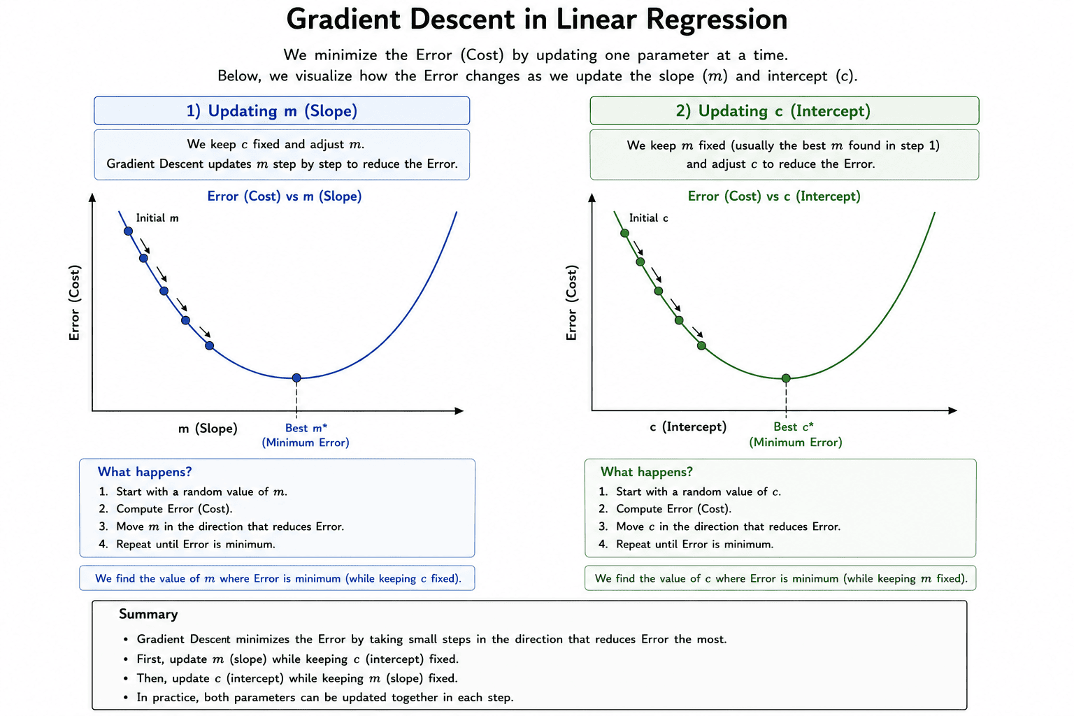
Gradient Descent is the "adjust and improve" strategy we described at the very start the blindfolded hiker feeling their way downhill, one step at a time.
At each step, the model:
- Checks how wrong its current guess is (using the cost function).
- Figures out which direction to nudge each setting to reduce that wrongness.
- Takes a small step in that direction.
- Repeats, thousands of times, until the wrongness stops improving much.
Unlike the Normal Equation, gradient descent doesn't need one big, expensive calculation it just needs lots of small, cheap ones. That's exactly why it works for huge models (like deep neural networks with millions of settings) where the Normal Equation would be hopeless.
https://hackernoon.com/dl03-gradient-descent-719aff91c7d6
Gradient Descent Variants
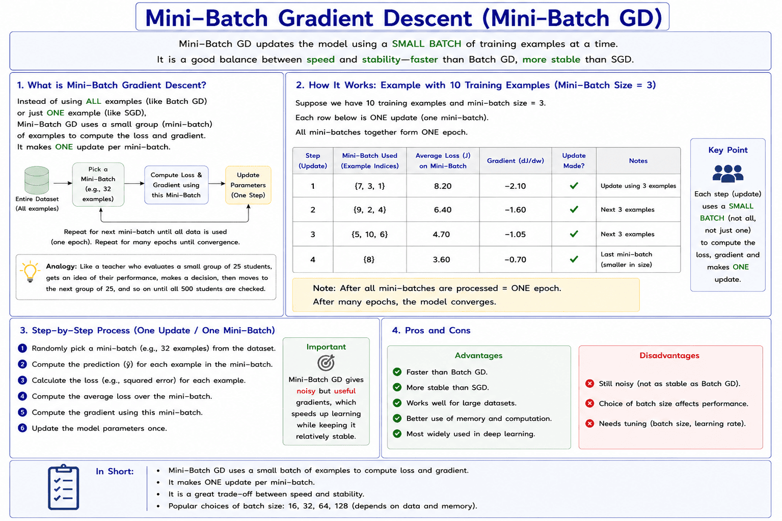
There's one important choice we haven't discussed yet. Suppose you have 10,000 training examples. When Gradient Descent calculates the loss, should it look at all 10,000 examples, just one randomly chosen example, or perhaps 100 examples at a time? Each choice creates a different variant of Gradient Descent.
Batch GD
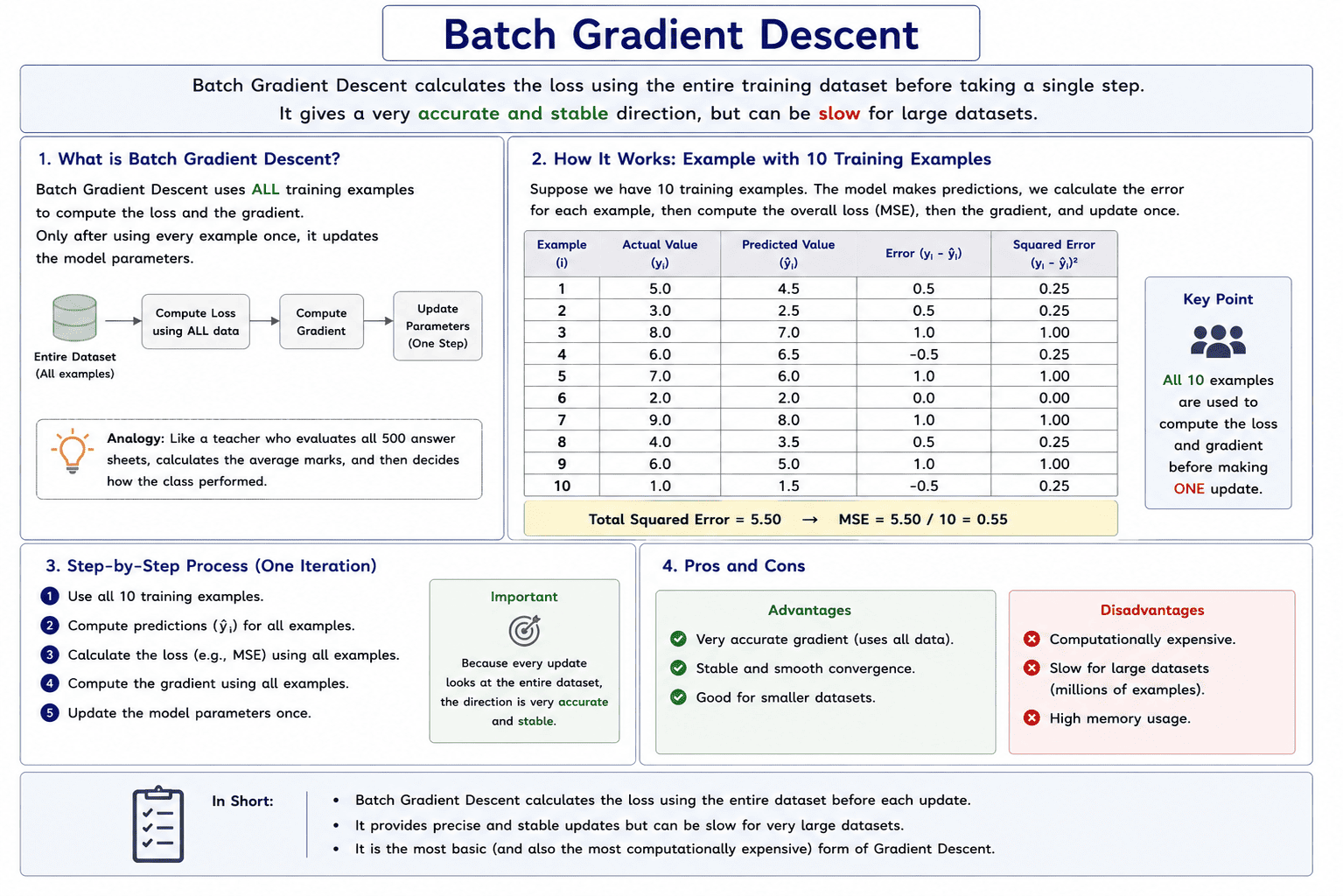
Batch Gradient Descent calculates the loss using the entire training dataset before taking a single step toward the minimum. For example, suppose you have a dataset containing 10,000 training examples. Before updating the model's parameters even once, Batch Gradient Descent first calculates the loss using all 10,000 examples, computes the gradient, and then makes a single update. Because every update is based on the complete dataset, the direction of the next step is very accurate and stable.
Think of it like a teacher who wants to know the average marks of a class with 500 students. Instead of checking just a few answer sheets, the teacher first evaluates all 500 papers, calculates the average score, and only then decides how the class performed. The result is highly accurate because every student's performance has been considered.
Batch Gradient Descent works in exactly the same way. It looks at every training example before deciding how to adjust the model. The drawback, however, is speed. If the dataset contains millions of examples, the algorithm must process every one of them before making each update. As a result, although Batch Gradient Descent is accurate and produces smooth, stable updates, it can become slow and computationally expensive for very large datasets.
SGD
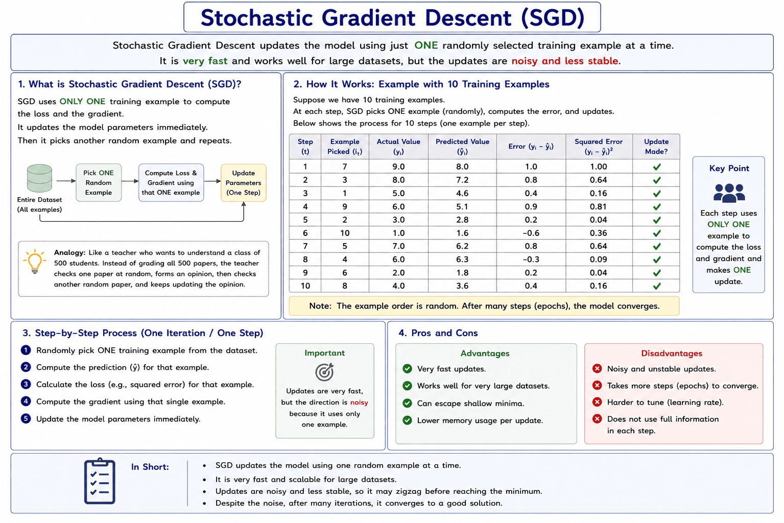
Stochastic Gradient Descent (SGD) takes a completely different approach. Instead of calculating the loss using the entire training dataset, it updates the model after looking at just one randomly selected training example. For example, suppose you have a dataset containing 10,000 training examples. Rather than evaluating all 10,000 examples before making an update, SGD randomly picks one example, calculates the loss and the gradient for that single example, and immediately updates the model's parameters. It then picks another random example, updates again, and continues this process until it has gone through the entire dataset.
Think of it like a teacher who wants to understand how well a class of 500 students is performing. Instead of grading all 500 answer sheets before forming an opinion, the teacher picks one answer sheet at random, reviews it, slightly adjusts their understanding of the class, then picks another random answer sheet and repeats the process. Each individual paper may not perfectly represent the whole class, so the teacher's opinion changes frequently. However, after reviewing many randomly selected papers over time, the teacher develops a fairly accurate understanding of the overall class performance.
Stochastic Gradient Descent works in exactly the same way. It updates the model after examining just one training example at a time, making each update extremely fast. This allows the algorithm to start learning almost immediately and makes it well suited for very large datasets. The drawback, however, is that each update is based on only one example, so the direction of the next step can be noisy and unstable. Instead of moving smoothly toward the minimum like Batch Gradient Descent, SGD often zigzags around the minimum before eventually converging. Despite this instability, its speed and ability to handle massive datasets make it one of the most widely used optimization techniques in machine learning.
Mini-Batch GD
Batch Gradient Descent (Batch GD) takes a systematic approach to optimizing a model. Instead of updating the model after every training example, it first calculates the loss using the entire training dataset and then performs one update to the model's parameters. For example, suppose you have a dataset containing 10,000 training examples. Before making even a single update, Batch Gradient Descent evaluates the loss for all 10,000 examples, computes the overall gradient, and then updates the model's parameters once. It repeats this process until the model reaches the minimum loss.
Think of it like a teacher who wants to understand how well a class of 500 students has performed in an exam. Instead of looking at just a few answer sheets, the teacher carefully grades all 500 papers, calculates the average marks of the class, and only then decides how the class performed. Since every student's performance has been considered, the teacher's conclusion is highly accurate and stable.
Batch Gradient Descent works in exactly the same way. It updates the model only after examining every training example, ensuring that each update is based on the complete dataset. This produces a very accurate and stable direction toward the minimum, resulting in smooth and predictable learning. The drawback, however, is speed. If the dataset contains millions of training examples, the algorithm must process every one of them before making each update. As a result, each iteration can take a considerable amount of time and require significant computational resources. Although Batch Gradient Descent is slower than its alternatives, its stable and accurate updates make it an excellent choice for small- to medium-sized datasets where computational cost is less of a concern.
Adaptive Optimizers
Adaptive Optimizers take Gradient Descent one step further by automatically adjusting the learning rate during training. Unlike Batch Gradient Descent or Stochastic Gradient Descent, which typically use the same learning rate for every update, adaptive optimizers modify the step size for each parameter based on how it has been learning. For example, suppose you are training a model with 10,000 training examples and millions of parameters. Instead of updating every parameter by the same amount (say 0.01), an adaptive optimizer may give a larger update to one parameter and a smaller update to another, depending on how each one is progressing. This allows the model to learn more efficiently and often reach the minimum loss faster.
Think of it like a teacher helping a class of 500 students prepare for an examination. Instead of giving every student the same amount of attention, the teacher focuses more on students who need extra help and less on those who are already performing well. By adjusting the guidance based on each student's progress, the teacher helps the entire class improve more effectively.
Adaptive optimizers work in exactly the same way. They monitor each parameter during training and automatically adjust its learning rate, leading to faster convergence and often better performance than traditional Gradient Descent. Some of the most popular adaptive optimizers are AdaGrad, RMSProp, Adam, and Momentum.
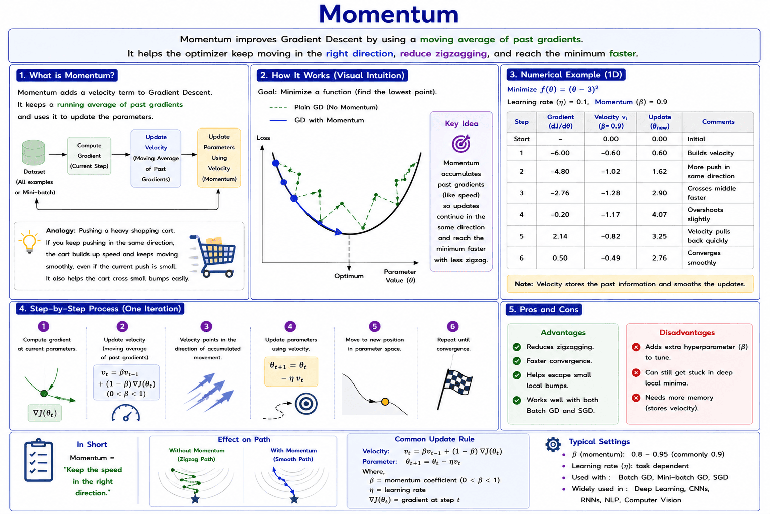
1) Momentum
Momentum improves Gradient Descent by remembering the direction of previous updates. Instead of starting from scratch after every iteration, it carries some "momentum" from earlier steps, allowing the model to move more smoothly toward the minimum.
Imagine pushing a heavy shopping cart in a supermarket. The first push requires effort, but once the cart is moving, it continues rolling in the same direction with less effort. Similarly, Momentum allows the optimizer to keep moving in the right direction instead of slowing down after every update.
Momentum helps reduce the zigzag movement often seen in Stochastic Gradient Descent, resulting in faster and smoother convergence. However, it still uses the same learning rate for every parameter, so it is not considered an adaptive optimizer.
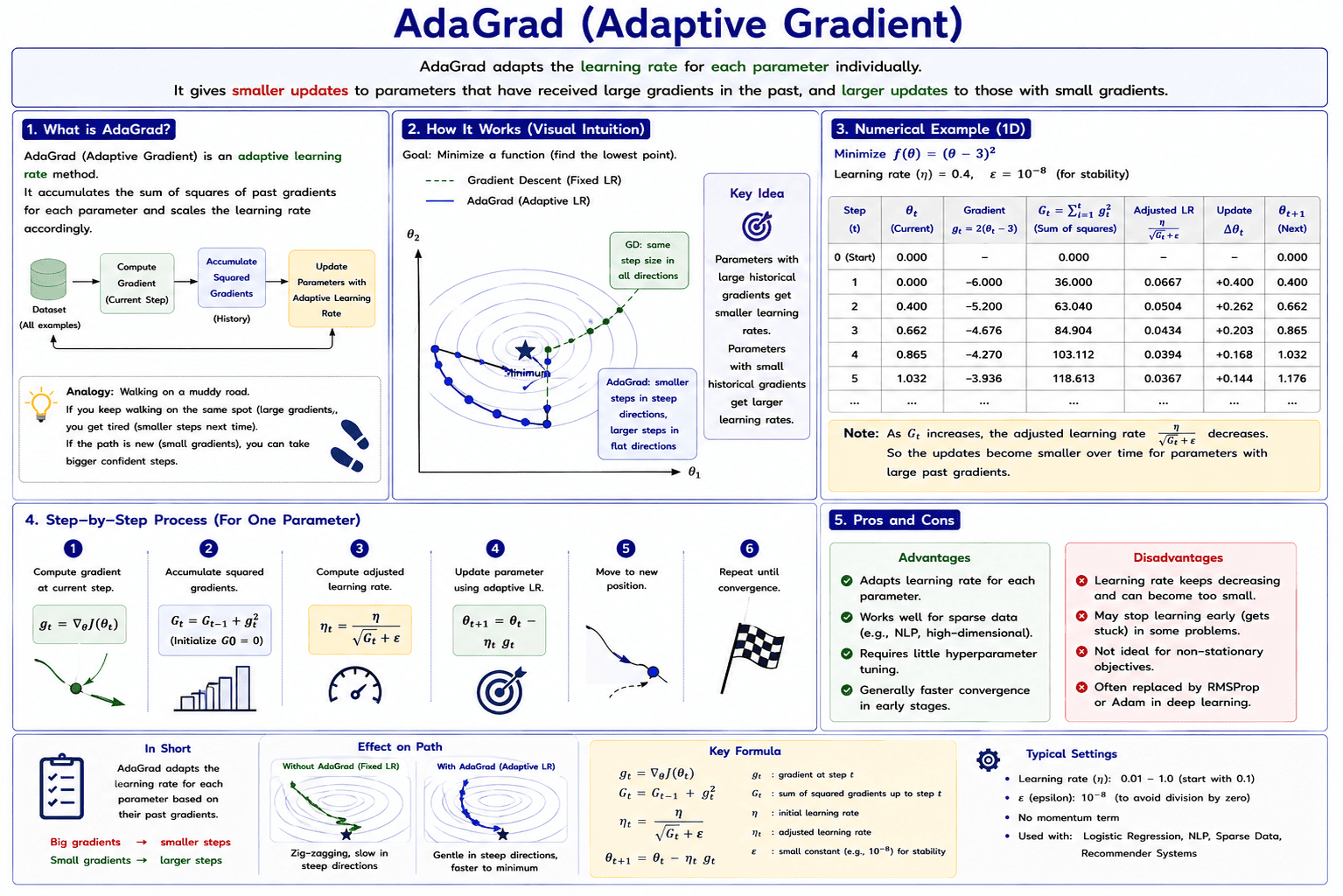
2) AdaGrad (Adaptive Gradient)
AdaGrad was the first optimizer to introduce the idea of adaptive learning rates. Instead of updating every parameter by the same amount, AdaGrad assigns a different learning rate to each parameter based on how frequently it has been updated.
Imagine a teacher helping students prepare for an exam. Students who frequently make mistakes receive smaller, more careful corrections over time, while students who have not been corrected much receive larger guidance. This allows each student to learn at a pace suited to their needs.
AdaGrad works in exactly the same way. Parameters that receive many updates gradually get smaller learning rates, while less frequently updated parameters continue to receive larger updates. This makes AdaGrad particularly useful for problems involving sparse data, such as text processing. However, its learning rates continually decrease and can eventually become so small that learning almost stops.
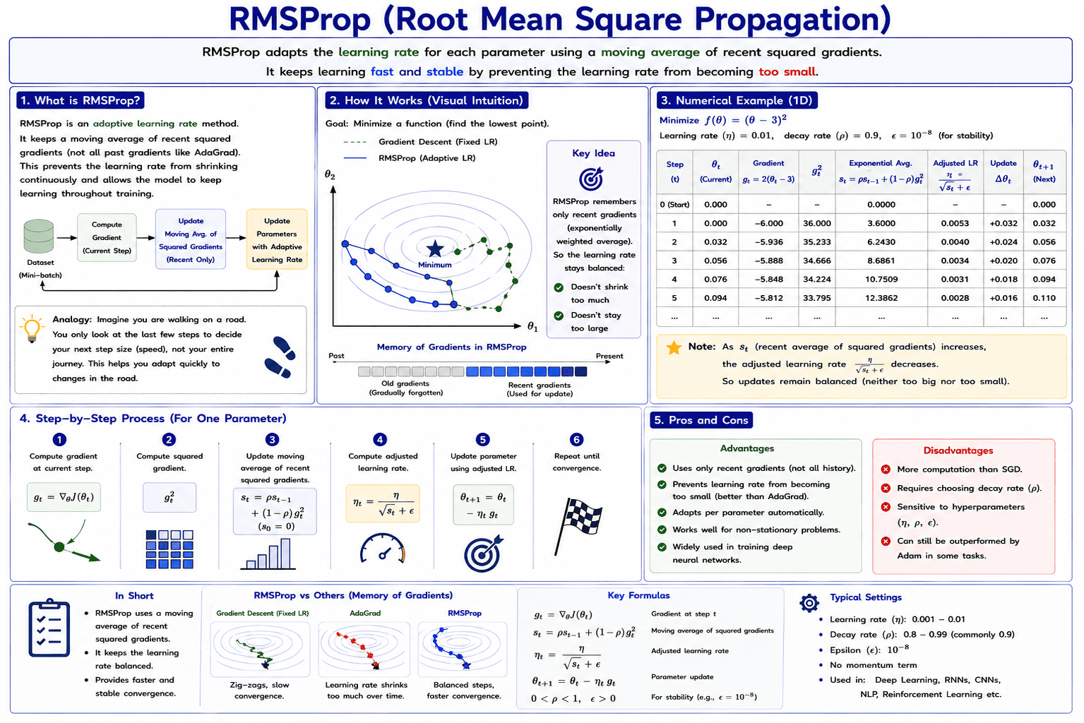
3) RMSProp (Root Mean Square Propagation)
RMSProp was developed to overcome AdaGrad's biggest limitation. Instead of allowing the learning rate to shrink forever, RMSProp keeps track of only the recent gradients and adjusts the learning rate accordingly.
Imagine a teacher who focuses mainly on a student's recent performance instead of every mistake the student has ever made. If a student improves, the teacher adjusts the guidance immediately rather than continuing to judge them based on old mistakes.
RMSProp behaves in the same way. By considering recent updates instead of the entire history, it prevents the learning rate from becoming excessively small. As a result, learning remains stable throughout training, making RMSProp well suited for deep learning and non-stationary problems.
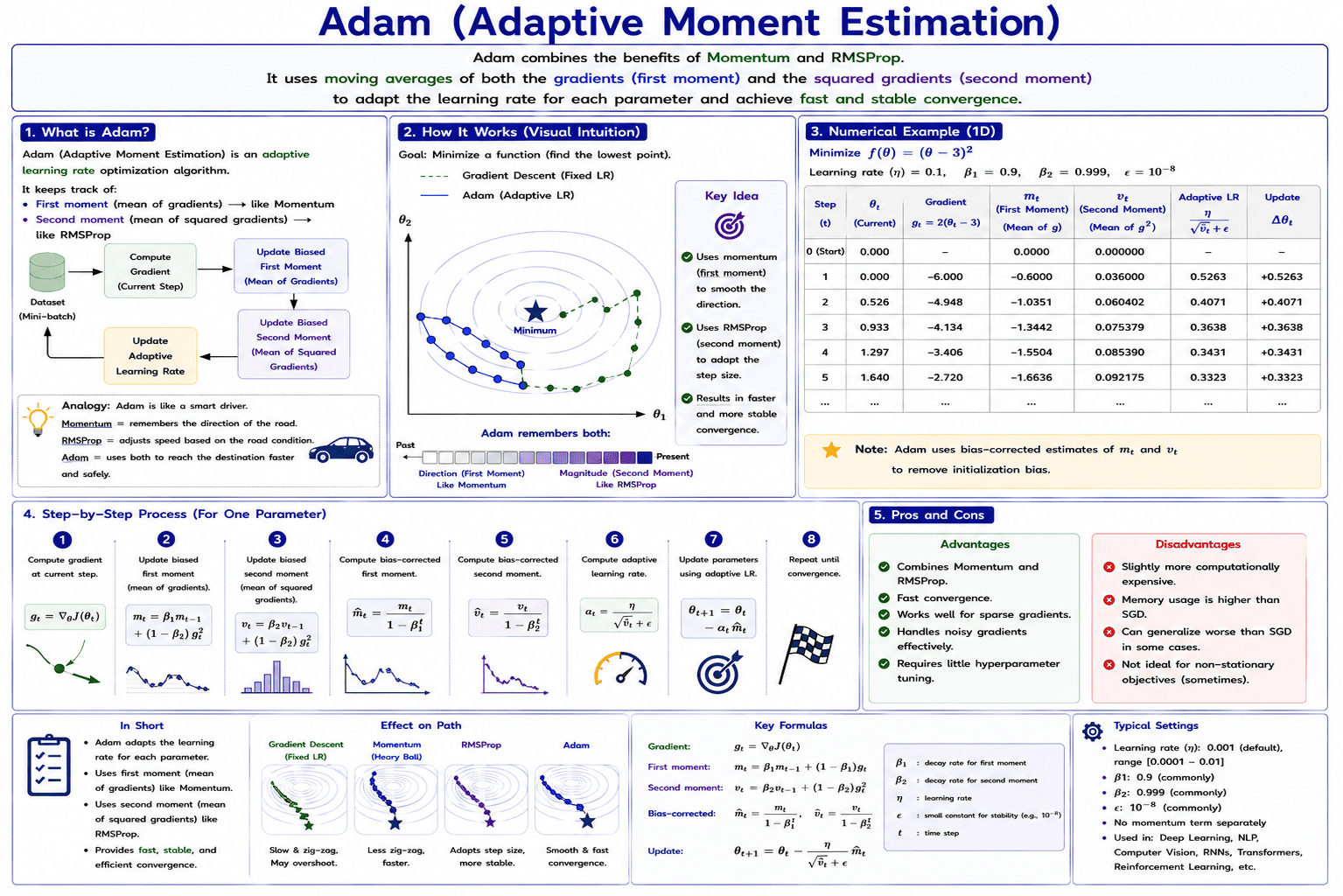
4. Adam (Adaptive Moment Estimation)
Adam combines the strengths of Momentum and RMSProp into a single optimization algorithm. It not only remembers the direction of previous updates (Momentum) but also adjusts the learning rate for each parameter (RMSProp).
Imagine an experienced teacher who not only remembers each student's past performance but also adjusts the amount of guidance based on how the student is performing now. Students who need more attention receive it, while those progressing well receive only minor corrections.
Adam works in exactly the same way. By combining momentum with adaptive learning rates, it usually converges faster than previous optimizers and requires very little manual tuning. Because of its speed, stability, and ease of use, Adam has become one of the most popular optimizers in machine learning and deep learning.
Tuning & Behavior
Learning Rate
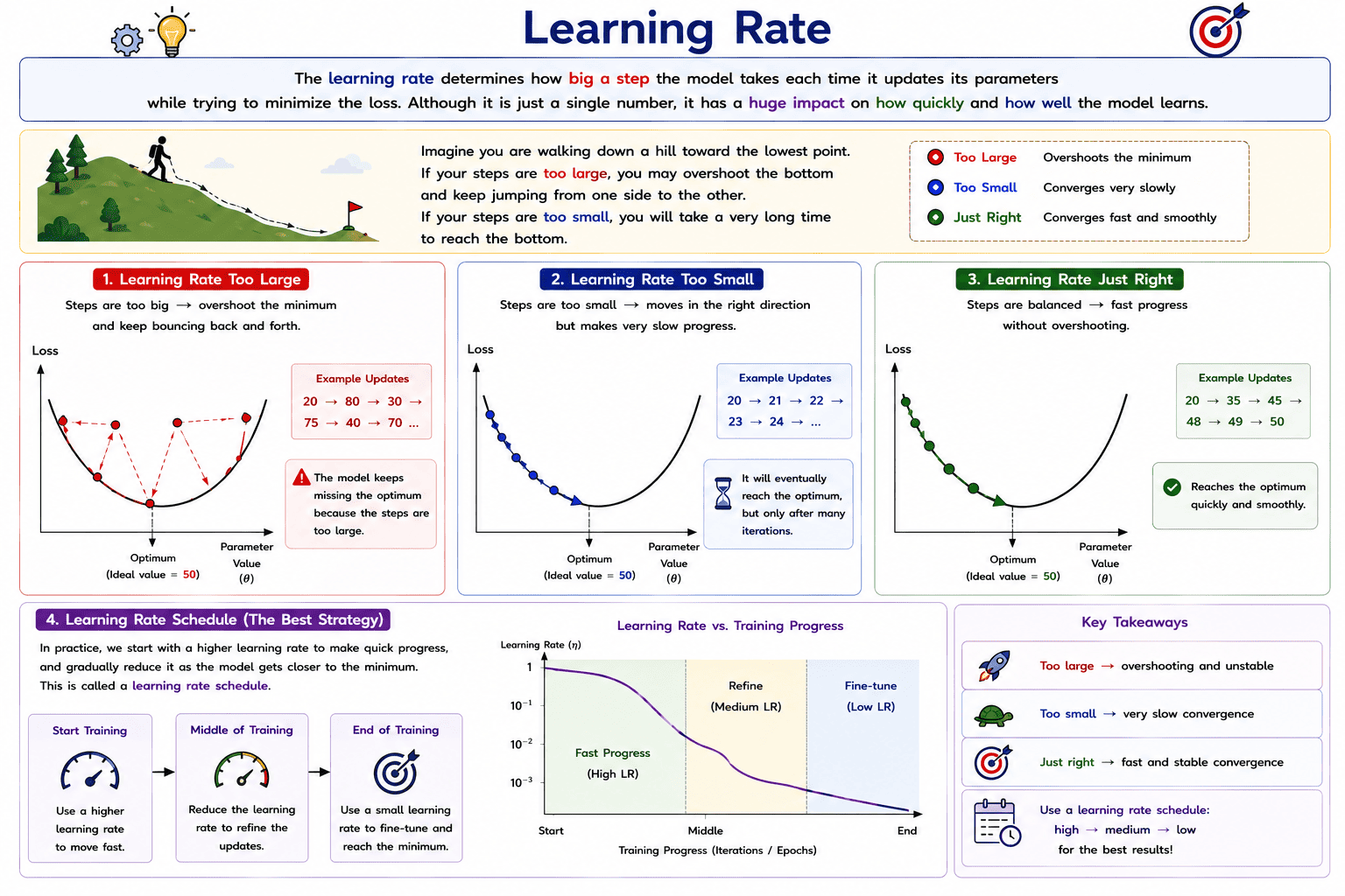
The learning rate determines how big a step the model takes each time it updates its parameters while trying to minimize the loss. Although it is just a single number, it has a huge impact on how quickly and how well the model learns.
Imagine you are walking down a hill toward the lowest point. If your steps are too large, you may overshoot the bottom and keep jumping from one side to the other. For example, if the ideal parameter value is 50, the updates might look like this:
20 → 80 → 30 → 75 → 40 → 70 ...
The model keeps missing the optimum because the steps are too large.
On the other hand, if the learning rate is too small, the model moves in the right direction but makes very slow progress:
20 → 21 → 22 → 23 → 24 ...
It will eventually reach the optimum, but only after many iterations.
The ideal learning rate is large enough to make fast progress but small enough to avoid overshooting the minimum. In practice, training often starts with a higher learning rate and gradually reduces it as the model gets closer to the minimum. This strategy is called a learning rate schedule, allowing the model to make quick progress initially and fine-tune its parameters toward the end of training.
Convergence
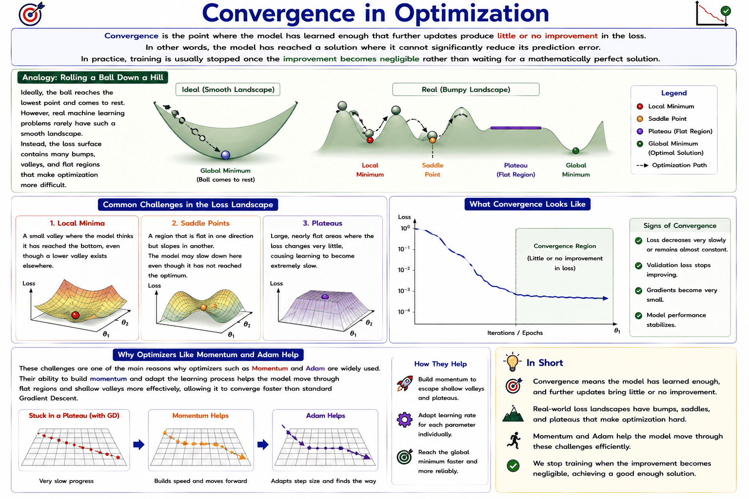
Convergence is the point where the model has learned enough that further updates produce little or no improvement in the loss. In other words, the model has reached a solution where it cannot significantly reduce its prediction error. In practice, training is usually stopped once the improvement becomes negligible rather than waiting for a mathematically perfect solution.
Imagine rolling a ball down a hill. Ideally, the ball reaches the lowest point and comes to rest. However, real machine learning problems rarely have such a smooth landscape. Instead, the loss surface contains many bumps, valleys, and flat regions that make optimization more difficult.
Some common challenges are:
- Local Minima: A small valley where the model thinks it has reached the bottom, even though a lower valley exists elsewhere.
- Saddle Points: A region that is flat in one direction but slopes in another. The model may slow down here even though it has not reached the optimum.
- Plateaus: Large, nearly flat areas where the loss changes very little, causing learning to become extremely slow.
These challenges are one of the main reasons why optimizers such as Momentum and Adam are widely used. Their ability to build momentum and adapt the learning process helps the model move through flat regions and shallow valleys more effectively, allowing it to converge faster than standard Gradient Descent.
Comparison
| Method | Type | Iterative? | Good for Large Data? | Speed per Step | Path to the Answer | Typically Used For |
|---|---|---|---|---|---|---|
| OLS / Normal Equation | Exact formula | No, One-shot | No | One-shot but expensive | Direct, exact | Small linear regression problems |
| Batch GD | Step-by-step | Yes | No | Slow | Smooth | Small datasets |
| SGD | Step-by-step | Yes | Yes | Very fast | Noisy, jumpy | Streaming / huge datasets |
| Mini-Batch GD | Step-by-step | Yes | Yes | Fast | Fairly smooth | Default for most model training |
| Momentum | Smarter steps | Yes | Yes | Fast | Smoother, faster | Deep learning |
| AdaGrad / RMSProp | Smarter steps | Yes | Yes | Fast | Adapts per setting | Sparse or uneven data |
| Adam | Smarter steps | Yes | Yes | Fast | Fast and reliable | Default for deep learning |