Decision Tree
Decision Tree
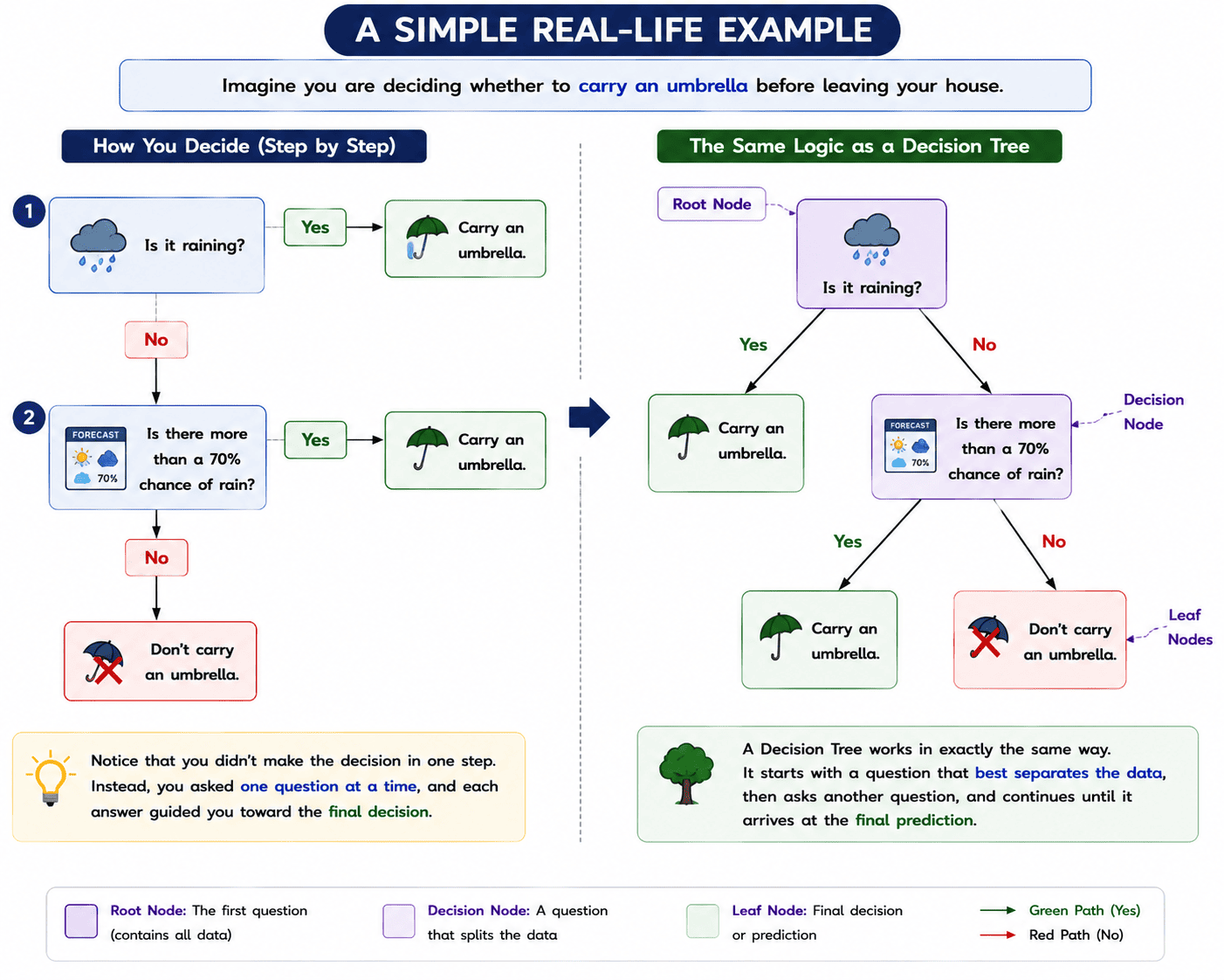
A Decision Tree is one of the simplest and most intuitive machine learning algorithms. It learns by asking a series of questions and uses the answers to make a prediction or decision.
Just as humans often make decisions step by step, a Decision Tree also reaches a conclusion by breaking a problem into a sequence of smaller decisions.
A Decision Tree is a Supervised Machine Learning algorithm, which means it learns from labeled training data. It can be used for both:
- Classification – predicting categories (e.g., Yes/No, Spam/Not Spam).
- Regression – predicting numerical values (e.g., house price, salary, temperature).
- Instead of trying to solve a problem all at once, a Decision Tree repeatedly divides the data into smaller groups by asking the most useful question at each step. This process continues until it reaches a final prediction.
Working of a Decision Tree
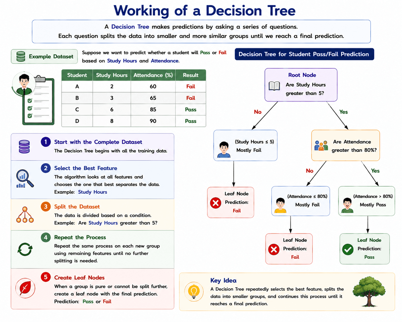
A Decision Tree works by asking a sequence of questions. Each question divides the dataset into smaller and more similar groups. This process continues until the tree reaches a final prediction.
Let's understand this with a simple example.
Example Dataset
Suppose we want to predict whether a student will Pass or Fail based on Study Hours and Attendance.
| Study Hours | Attendance (%) | Result |
|---|---|---|
| 2 | 60 | Fail |
| 3 | 65 | Fail |
| 6 | 85 | Pass |
| 8 | 90 | Pass |
Step 1: Start with the Complete Dataset
The Decision Tree begins with the entire training dataset. At this stage, the data contains both Pass and Fail records, so the tree cannot make a prediction.
Step 2: Select the Best Feature
The algorithm examines all the available features, such as Study Hours and Attendance, and chooses the one that best separates the data into different groups.
In this example, suppose the algorithm selects Study Hours as the first feature.
Step 3: Split the Dataset
The dataset is divided based on the selected feature. For example, the tree may ask:
"Are the Study Hours greater than 5?"
This creates two smaller groups—one containing students who studied more than 5 hours and the other containing students who studied 5 hours or less.
Step 4: Repeat the Process
If a group still contains both Pass and Fail records, the Decision Tree asks another question using the remaining features.
For example, it may next ask:
"Is the Attendance greater than 80%?"
The tree continues asking questions and splitting the data until each group becomes sufficiently pure.
Step 5: Create Leaf Nodes
When no further splitting is required, the process stops. The final nodes, called Leaf Nodes, contain the model's prediction.
For this example, the final prediction is either Pass or Fail.
A Decision Tree works by repeatedly selecting the best feature, splitting the data into smaller groups, and continuing this process until it reaches a final prediction.
Why is it Called a Decision Tree?
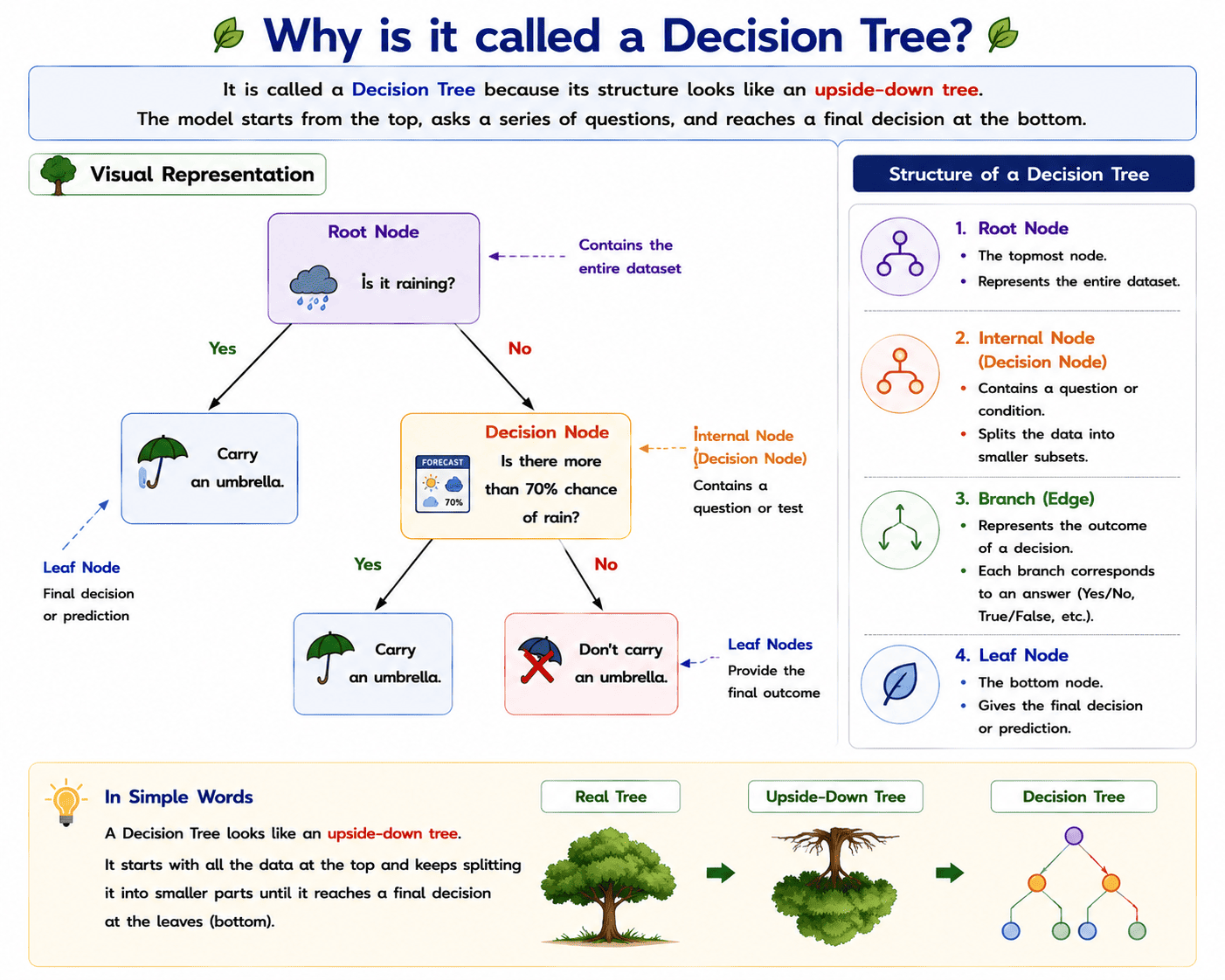
A Decision Tree is named after its tree-like structure. Just as a real tree starts with a single trunk and branches out into smaller branches, a Decision Tree starts with the entire dataset and repeatedly splits it into smaller groups by asking a series of questions. Each split creates a new branch, and the process continues until the final prediction is reached at the leaf nodes. Because it follows this branching pattern to make decisions, it is called a Decision Tree.
How Does a Decision Tree Decide the Best Split?
At every step, a Decision Tree must decide which feature should be used to split the data first. But how does it make this decision?
Consider the student dataset used earlier. Suppose the available features are:
- Study Hours
- Attendance
- Age
The Decision Tree could split the data using any of these features. For example, it could ask:
- Are Study Hours greater than 5?
- Is Attendance greater than 80%?
- Is Age greater than 18 years?
However, not every question produces a good split. Some questions may separate the Pass and Fail students very clearly, while others may still leave both classes mixed together. Naturally, the Decision Tree prefers the question that creates the cleanest and most meaningful separation of the data.
To determine which split is the best, Decision Trees use mathematical measures known as splitting criteria. These criteria evaluate every possible split and select the one that separates the data most effectively.
The most commonly used splitting criteria are:
- Entropy
- Information Gain
- Gini Index
- Variance Reduction (used in regression trees)
Entropy
Suppose we want to build a Decision Tree to predict whether a student will Pass or Fail.
Consider the following dataset.
| Student | Study Hours | Attendance (%) | Age | Result |
|---|---|---|---|---|
| A | 2 | 60 | 18 | Fail |
| B | 3 | 65 | 19 | Fail |
| C | 4 | 70 | 20 | Fail |
| D | 6 | 75 | 19 | Pass |
| E | 7 | 85 | 21 | Pass |
| F | 8 | 90 | 22 | Pass |
The Decision Tree now has to decide which feature should be used to split the data first.
The possible features are:
- Study Hours
- Attendance
- Age
At first glance, all three seem like reasonable choices. But which one should the Decision Tree select?
Suppose the tree evaluates each feature and obtains the following groups.
Split using Study Hours
| Study Hours ≤ 5 | Study Hours > 5 |
|---|---|
| Fail, Fail, Fail | Pass, Pass, Pass |
This split produces two completely pure groups.
Split using Attendance
| Attendance ≤ 75 | Attendance > 75 |
|---|---|
| Fail, Fail, Fail, Pass | Pass, Pass |
The left group still contains both Pass and Fail students, so it is not completely pure.
Split using Age
| Age ≤ 20 | Age > 20 |
|---|---|
| Fail, Fail, Fail, Pass | Pass, Pass |
This split also leaves a mixed group and is therefore less effective.
Now the question is, How does the Decision Tree know that splitting on Study Hours is better than splitting on Attendance or Age?
It needs a way to measure how pure or impure the groups become after each possible split.
This measure is called Entropy.
What is Entropy?
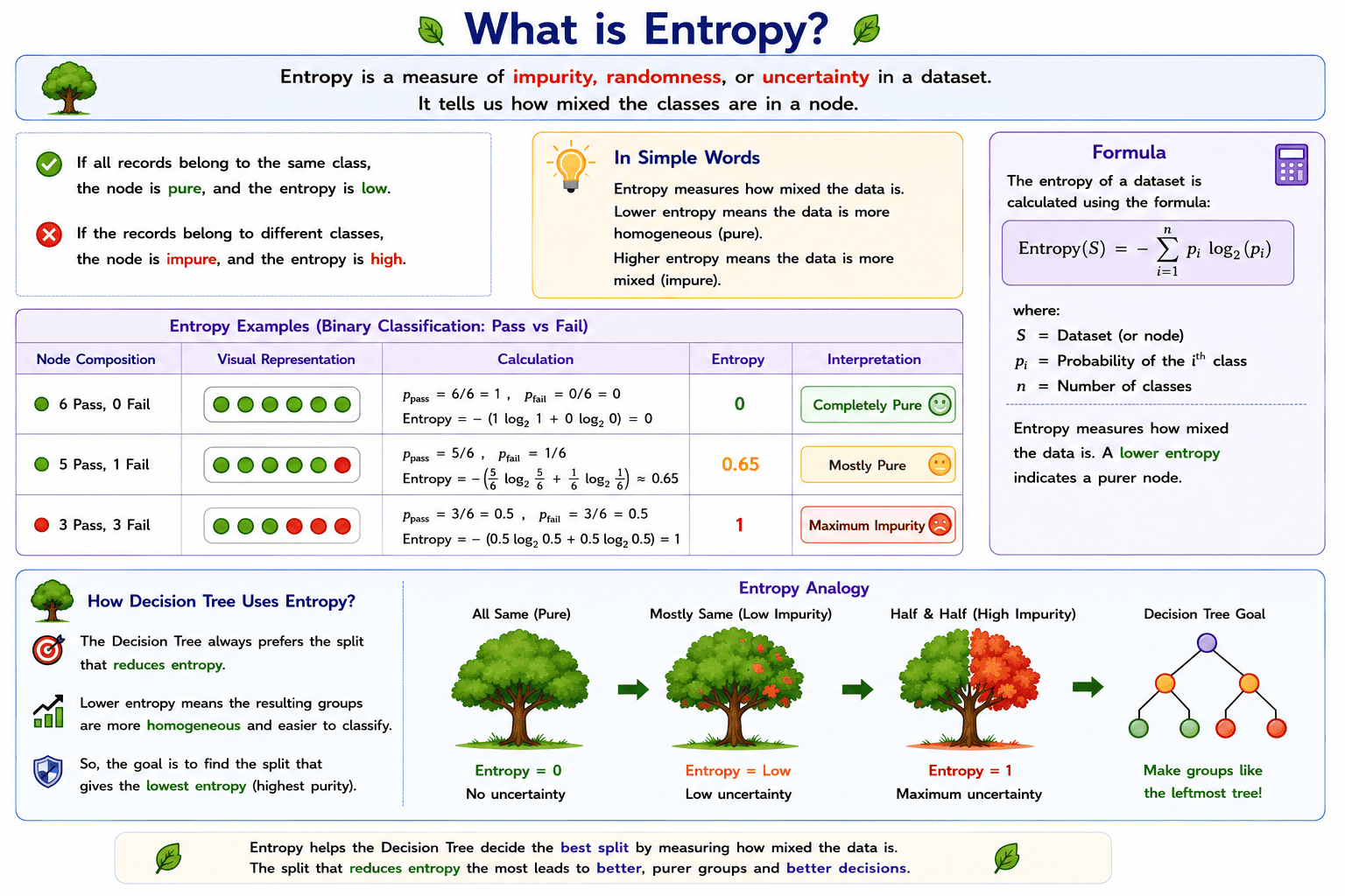
Entropy is a measure of impurity, randomness, or uncertainty in a dataset. It tells us how mixed the classes are in a node.
- If all records belong to the same class, the node is pure, and the entropy is low.
- If the records belong to different classes, the node is impure, and the entropy is high.
For a binary classification problem:
| Node Composition | Entropy | Interpretation |
|---|---|---|
| 6 Pass, 0 Fail | 0 | Completely Pure |
| 5 Pass, 1 Fail | Low | Mostly Pure |
| 3 Pass, 3 Fail | 1 | Maximum Impurity |
Thus,
- Entropy = 0 means there is no uncertainty because every record belongs to the same class.
- Entropy = 1 means there is maximum uncertainty because the classes are equally mixed.
The Decision Tree always prefers the split that reduces entropy, because lower entropy means the resulting groups are more homogeneous and easier to classify.
Formula
The entropy of a dataset is calculated using the following formula:
\[\text{Entropy}(S) = -\sum_{i=1}^{n} p_i \log_{2}(p_i)\]
where:
- S = Dataset (or node)
- pᵢ = Probability of the ith class
Entropy measures how mixed the data is. A lower entropy indicates a purer node, so a Decision Tree always prefers the split that produces the lowest entropy.
I agree. The previous version is too conversational. A textbook should read in a more formal, instructional style with short explanatory paragraphs instead of directly addressing the reader. Here's a version that would fit naturally in a Machine Learning or Decision Tree chapter.
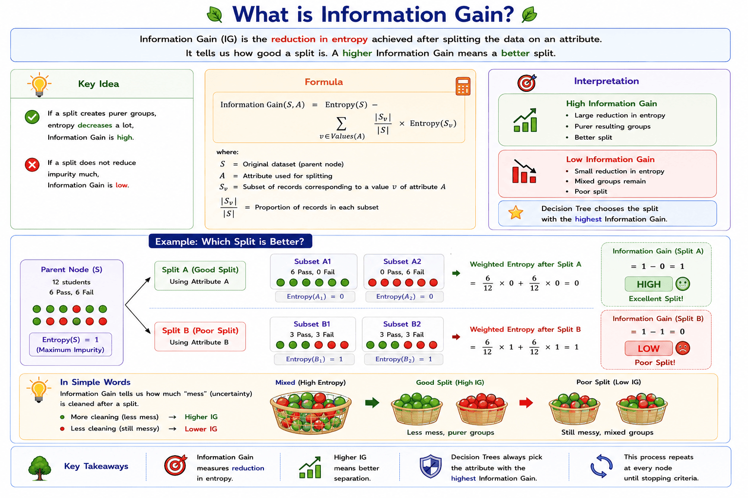
What is Information Gain?
While Entropy measures the impurity or uncertainty present in a dataset, it does not indicate which attribute should be selected for splitting the data. This decision is made using Information Gain.
Information Gain is a criterion used by Decision Tree algorithms to evaluate the effectiveness of a split. It measures the reduction in entropy obtained after partitioning the dataset using a particular attribute. A split that produces more homogeneous subsets results in a higher Information Gain.
The objective of a Decision Tree is to create nodes that contain records belonging to the same class as much as possible. Therefore, at every stage of the tree construction, the algorithm evaluates all possible attributes and selects the one that provides the highest Information Gain.
Definition
Information Gain is the reduction in entropy achieved after splitting a dataset on a particular attribute. It indicates how well an attribute separates the training data into distinct classes.
Interpretation
The value of Information Gain depends on the quality of the split produced by an attribute.
- A high Information Gain indicates that the split has significantly reduced the impurity of the dataset. The resulting child nodes are more homogeneous and contain records that mostly belong to the same class.
- A low Information Gain indicates that the split has not reduced the impurity considerably. The child nodes remain mixed, making them less useful for classification.
Consequently, the attribute with the highest Information Gain is selected for splitting the node.
Formula
Information Gain is calculated as the difference between the entropy of the parent node and the weighted average entropy of the child nodes.
\[\text{Information Gain}(S, A)=\text{Entropy}(S)-\sum_{v \in \text{Values}(A)}\frac{|S_v|}{|S|}\cdot\text{Entropy}(S_v)\]
where
- (S) represents the original dataset (parent node).
- (A) represents the attribute used for splitting.
- (S_v) represents the subset of records corresponding to a particular value of the attribute.
- (|S_v|/|S|) represents the proportion of records in each subset.
The first term represents the impurity before the split, while the second term represents the impurity remaining after the split. Their difference gives the Information Gain.
Working Principle
The process of selecting the best split in a Decision Tree can be summarized as follows.
- Compute the entropy of the parent node.
- Split the dataset using each candidate attribute.
- Calculate the entropy of each resulting child node.
- Compute the weighted average entropy after the split.
- Determine the Information Gain for every attribute.
- Select the attribute with the highest Information Gain.
- Repeat the same process recursively until a stopping criterion is reached.
Illustrative Example
Consider a dataset containing an equal number of Pass and Fail records. Two different attributes are available for splitting the data.
Suppose Attribute A separates almost all Pass records into one group and most Fail records into another. Since the resulting subsets are nearly pure, the reduction in entropy is large, leading to a high Information Gain.
On the other hand, Attribute B produces two subsets that still contain a mixture of Pass and Fail records. In this case, the entropy remains relatively high, resulting in a low Information Gain.
The Decision Tree therefore selects Attribute A, as it provides a better separation of the classes.
Relationship Between Entropy and Information Gain
Entropy and Information Gain are complementary measures used during Decision Tree construction. Entropy quantifies the impurity present in a node, whereas Information Gain quantifies the reduction in impurity obtained after splitting that node.
Thus, Information Gain cannot be computed without first calculating entropy. The effectiveness of a split is determined by the amount of entropy it removes from the dataset.
Key Points
- Information Gain is used to select the best attribute for splitting a node.
- It measures the reduction in entropy after partitioning the dataset.
- A higher Information Gain indicates a more effective split.
- Decision Tree algorithms always prefer the attribute with the highest Information Gain.
- Repeated selection of attributes with maximum Information Gain results in a tree containing increasingly homogeneous nodes.
I agree. Since you're writing a textbook for beginners, the language should be simple, clear, and educational, not like a research paper. It should be easy enough for a second- or third-year undergraduate student to understand.
Here's a simpler version that still looks like a textbook chapter.
Gini Index
After understanding Entropy and Information Gain, let us learn another important measure used in Decision Trees called the Gini Index.
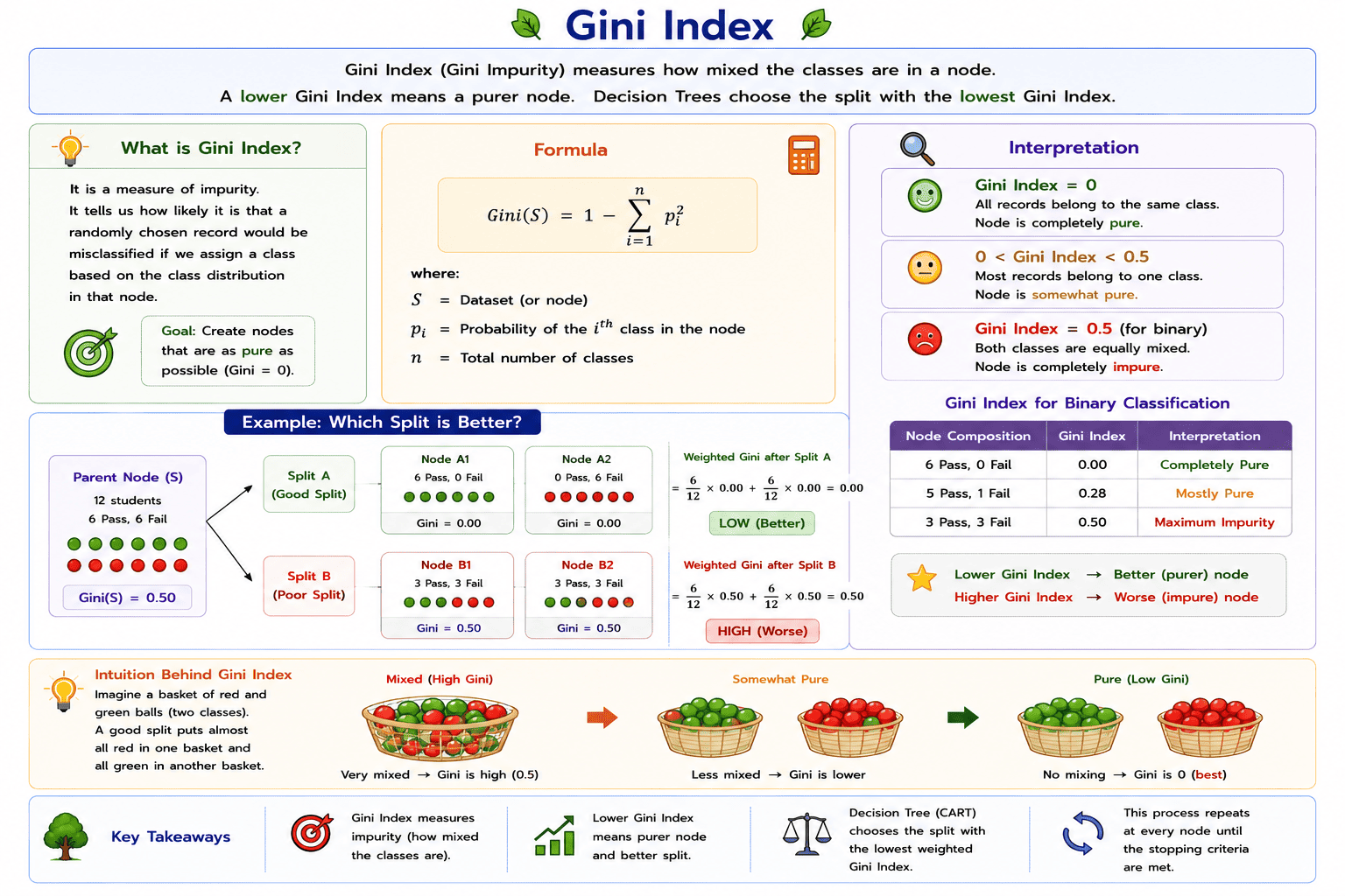
The Gini Index, also known as Gini Impurity, measures how mixed the classes are in a node. In simple words, it tells us whether the records in a node mostly belong to one class or are evenly distributed among different classes.
If all the records belong to the same class, the node is pure, and the Gini Index is 0. If the records are evenly divided among different classes, the node becomes impure, and the Gini Index increases.
Just like Information Gain, the Gini Index is used to find the best split in a Decision Tree. However, instead of choosing the split with the highest Information Gain, it chooses the split with the lowest Gini Index.
Definition
The Gini Index is a measure of impurity that shows how mixed the classes are in a dataset or node. A lower Gini Index indicates a purer node, while a higher Gini Index indicates a more impure node.
The Gini Index is a measure of impurity used in Decision Trees. It measures how mixed the classes are in a node, and the best split is the one that produces the lowest Gini Index.
Interpretation
The value of the Gini Index helps us understand the purity of a node.
- Gini Index = 0 means all the records belong to the same class. The node is completely pure.
- A low Gini Index means most of the records belong to one class. The node is nearly pure.
- A high Gini Index means the records belong to different classes. The node is impure.
- In a binary classification problem, the maximum Gini Index is 0.5, which occurs when both classes are equally mixed.
Therefore, a Decision Tree always tries to create nodes with the lowest possible Gini Index.
Formula
The Gini Index is calculated using the following formula:
\[\text{Gini}(S)=1-\sum_{i=1}^{n}p_i^2\]
where
- (S) is the dataset (or node).
- (pi) is the probability of the (ith) class.
- (n) is the total number of classes.
The formula calculates the impurity of the node. A lower Gini value indicates that the node contains records from mostly one class.
Example
Consider a binary classification problem involving Pass and Fail students.
| Node Composition | Gini Index | Interpretation |
|---|---|---|
| 6 Pass, 0 Fail | 0.00 | Completely Pure |
| 5 Pass, 1 Fail | 0.28 | Mostly Pure |
| 3 Pass, 3 Fail | 0.50 | Maximum Impurity |
From the above table, it can be observed that the Gini Index increases as the classes become more evenly mixed. A completely pure node has a Gini Index of 0, while a node containing equal numbers of both classes has the highest Gini value in binary classification.
How Does a Decision Tree Use the Gini Index?
During the construction of a Decision Tree, the algorithm calculates the Gini Index for every possible split.
The split that produces the lowest weighted Gini Index is selected because it creates child nodes that are more homogeneous. This process continues until the stopping criteria are met.
Relationship Between Entropy and Gini Index
Both Entropy and Gini Index measure the impurity of a node.
The main difference is that Entropy uses logarithms in its calculation, whereas the Gini Index uses squared probabilities. Although the formulas are different, both measures are used to identify the best split in a Decision Tree.
The ID3 algorithm uses Entropy and Information Gain, while the CART algorithm uses the Gini Index as its splitting criterion.
Key Points
- The Gini Index measures how mixed the classes are in a node.
- A Gini Index of 0 indicates a completely pure node.
- Lower Gini values indicate better splits.
- Decision Trees always choose the split with the lowest weighted Gini Index.
- The Gini Index is the splitting criterion used by the CART algorithm.
Types of Decision Trees
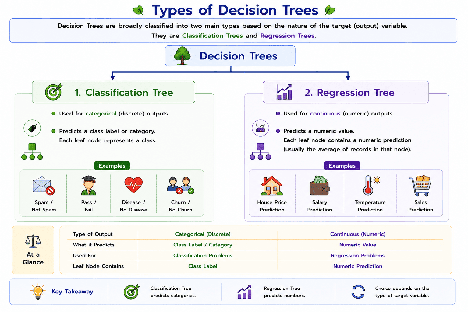
Decision Trees are classified into two main types based on the type of output they predict: Classification Trees and Regression Trees.
1. Classification Tree
A Classification Tree is used when the target variable is categorical. It predicts the class or category to which a record belongs. The decision tree divides the data into different groups until each leaf node represents a specific class.
Some common applications of Classification Trees include email spam detection, student result prediction, disease diagnosis, customer churn prediction, and loan approval prediction.
Examples:
- Spam / Not Spam
- Pass / Fail
- Disease / No Disease
- Loan Approved / Rejected
2. Regression Tree
A Regression Tree is used when the target variable is continuous. Instead of predicting a class, it predicts a numerical value. The tree divides the data into smaller groups, and each leaf node contains a predicted numeric value.
Regression Trees are widely used for predicting quantities such as prices, salaries, temperatures, and sales.
Examples:
- House Price Prediction
- Salary Prediction
- Temperature Prediction
- Sales Forecasting
Classification Tree vs. Regression Tree
The main difference between the two types of Decision Trees lies in the type of output they produce. A Classification Tree predicts a category or class label, whereas a Regression Tree predicts a continuous numerical value. The choice of tree depends entirely on the nature of the target variable being predicted.
If the output variable is categorical, a Classification Tree is used. If the output variable is continuous, a Regression Tree is used.
This topic is best kept simple and intuitive because hyperparameters are introduced for the first time here. Here's a textbook-style version.
Hyperparameters in Decision Trees
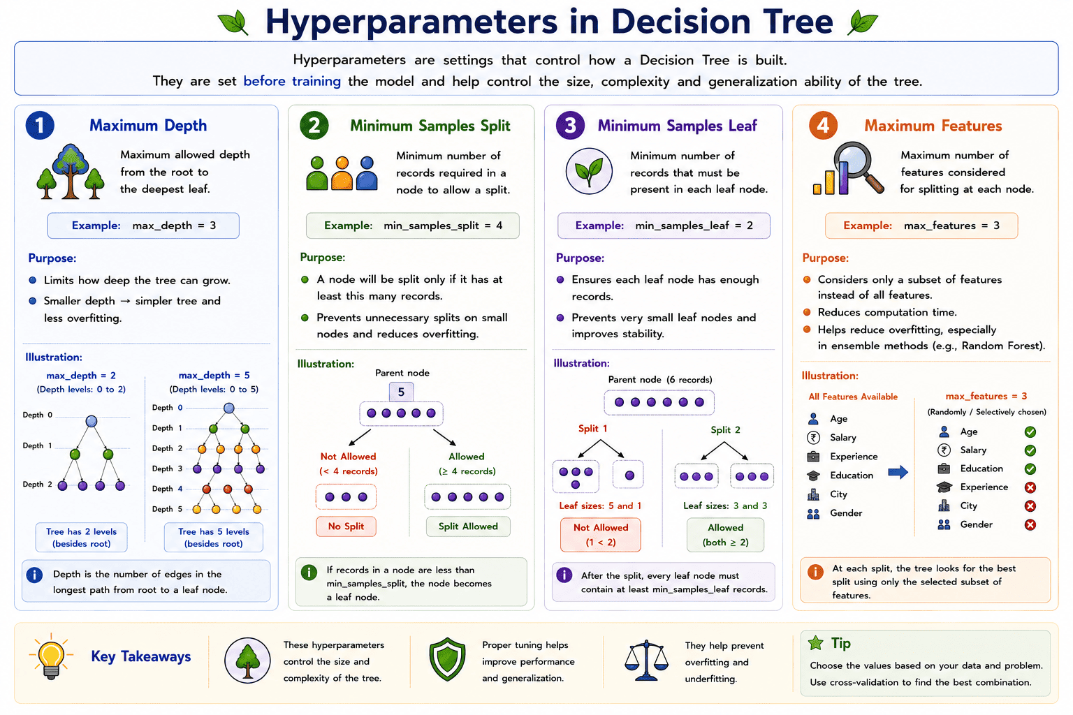
A hyperparameter is a setting that controls how a Decision Tree is built. These values are specified before training the model and help determine the structure, size, and complexity of the tree. Choosing appropriate hyperparameter values improves the performance of the model and helps prevent problems such as overfitting and underfitting.
The following are some of the most commonly used hyperparameters in Decision Trees.
1. Maximum Depth (max_depth)
The maximum depth specifies the maximum number of levels that a Decision Tree is allowed to grow.
A smaller depth creates a simpler tree, while a larger depth creates a more complex tree. Limiting the depth helps prevent the model from learning unnecessary details from the training data.
Example:
max_depth = 5
Purpose:
- Controls the depth of the tree.
- Helps prevent overfitting.
- Produces a simpler and more generalizable model.
2. Minimum Samples Split (min_samples_split)
The minimum samples split specifies the minimum number of records required for a node to be divided into two child nodes.
If a node contains fewer records than this value, it is not split further.
Example:
min_samples_split = 4
Purpose:
- Prevents unnecessary splitting.
- Reduces the complexity of the tree.
- Helps avoid overfitting.
3. Minimum Samples Leaf (min_samples_leaf)
The minimum samples leaf specifies the minimum number of records that must be present in every leaf node.
This ensures that leaf nodes do not contain very few observations.
Example:
min_samples_leaf = 2
Purpose:
- Prevents very small leaf nodes.
- Produces more stable predictions.
- Improves the generalization of the model.
4. Maximum Features (max_features)
The maximum features parameter specifies the maximum number of input features that are considered while searching for the best split at each node.
Instead of evaluating all available features, the algorithm considers only the specified number of features.
Example:
max_features = 3
Purpose:
- Reduces computation time.
- Introduces randomness during tree construction.
- Helps reduce overfitting, especially in ensemble methods such as Random Forest.
Key Points
- Hyperparameters are settings chosen before training a Decision Tree.
- They control the size, shape, and complexity of the tree.
- Proper tuning of hyperparameters improves model performance.
- Hyperparameters help reduce overfitting and improve the model's ability to generalize to new data.
Note: Choosing appropriate hyperparameter values is an important step in building an accurate and reliable Decision Tree model.
Overfitting in Decision Trees
A Decision Tree learns by creating rules that separate the data into different groups. If the tree is allowed to grow without any restrictions, it may become too complex and start learning the noise or random patterns present in the training data instead of the actual relationships.
This problem is known as overfitting. An overfitted Decision Tree performs very well on the training data but performs poorly on new or unseen data because it memorizes the training examples rather than learning general patterns.
A very deep Decision Tree usually indicates a higher risk of overfitting. Therefore, controlling the size and complexity of the tree is essential for building a model that generalizes well.
Example
Very Deep Tree
      ↓
Memorizes Training Data
      ↓
Poor Performance on New Data
Techniques to Prevent Overfitting
Several techniques can be used to reduce overfitting in Decision Trees.
- Pruning
- Limiting the maximum depth of the tree
- Setting the minimum number of samples required for splitting or leaf nodes
- Using ensemble methods such as Random Forest
Advantages of Decision Trees
Decision Trees are one of the most widely used machine learning algorithms because they are simple, easy to interpret, and can solve a variety of prediction problems.
- Easy to understand and visualize.
- Suitable for both classification and regression tasks.
- Can handle both numerical and categorical data.
- Requires very little data preprocessing.
- Feature scaling is generally not required.
- Produces decision rules that are easy to interpret.
Disadvantages of Decision Trees
Although Decision Trees offer several advantages, they also have some limitations that should be considered while building predictive models.
- Can easily overfit the training data.
- Sensitive to small changes in the dataset.
- Deep trees become difficult to interpret.
- May become computationally expensive for very large datasets.
- Different training datasets may produce different tree structures.
Real-World Applications of Decision Trees
Decision Trees are widely used across various industries because they are accurate, interpretable, and easy to implement.
Some common applications include:
- Fraud Detection
- Medical Diagnosis
- Loan Approval Systems
- Customer Segmentation
- Credit Risk Analysis
- Sales Prediction
- Employee Attrition Prediction
- Recommendation Systems
Note:Decision Trees are simple and powerful machine learning models. However, controlling the complexity of the tree using appropriate hyperparameters is important to prevent overfitting and improve the model's performance on unseen data.