Linear Regression
Linear Regression
Linear Regression is one of the most widely used Supervised Machine Learning algorithms for predicting continuous numerical values. It helps us understand how a change in one variable affects another variable by establishing a mathematical relationship between them.
In Linear Regression, the algorithm learns from historical data and identifies a pattern that can be used to make future predictions. The relationship between the input variables (features) and the output variable (target) is represented using a straight line known as the best-fit line.
Understanding the Idea of Linear Regression
The basic concept of Linear Regression is to learn the relationship between an input and an output variable.
For example, consider the relationship between study hours and examination marks. Generally, students who spend more time studying tend to score higher marks. By analyzing past data, the model can estimate how marks are likely to change as study hours increase or decrease.Student Marks Prediction
| Study Hours | Marks |
|---|---|
| 2 | 35 |
| 4 | 55 |
| 6 | 70 |
| 8 | 90 |
| 7 | 84 |
Once the relationship is learned, the model can predict the marks of a student based on the number of hours studied.
Real-World Applications of Linear Regression
Linear Regression is commonly used in many practical situations where numerical predictions are required.
| Input Variable | Output Variable |
|---|---|
| House Area | House Price |
| Study Hours, 10th%, 12th% marks | Examination Marks |
| Years of Experience, Performace | Salary |
| Temperature | Ice Cream Sales |
| Advertising Cost | Product Sales |
For instance, a real estate company can use Linear Regression to estimate the price of a house based on its size, while a business can predict product sales based on advertising expenditure.
Objectives of Linear Regression
The primary objectives of Linear Regression are:
- To predict continuous numerical values based on available data.
- To identify and measure the relationship between input and output variables.
- To understand how changes in one variable influence another variable.
- To minimize prediction errors by finding the line that best represents the data.
- To support decision-making by providing accurate forecasts and trends.
Relationship Between Regression Types
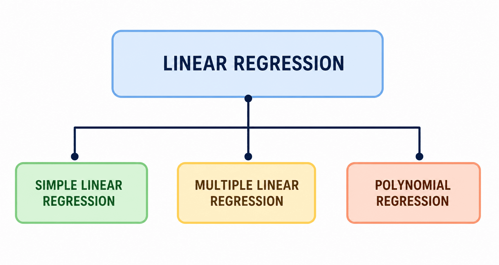
1. Simple Linear Regression
What is Simple Linear Regression?
Simple Linear Regression is a supervised machine learning algorithm used to predict a continuous numerical value. It learns the relationship between one input variable and one output variable by fitting a straight line through the data points.
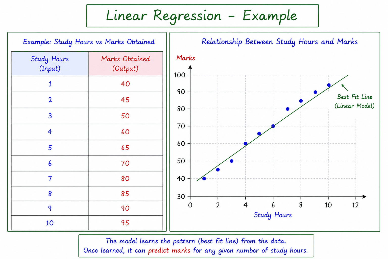
The diagram illustrates the relationship between Study Hours and Marks Obtained. As the number of study hours increases, the marks generally increase as well. Linear Regression learns this pattern from the data and uses it to make predictions for new values.
Example
In the diagram:
Input (X) -> Output (Y)
Independent Variable (X) -> Dependent Variable (Y)
Study Hours -> Marks Obtained
The table on the left contains historical data showing how many hours students studied and the marks they scored. The graph on the right plots these values as points and draws a straight line representing the relationship between the two variables.
Linear Regression Equation
The relationship between the input and output is represented by the equation:
\[y = mx + c\]
Meaning of Terms
| Symbol | Meaning |
|---|---|
| y | Output or Target Variable |
| x | Input or Feature Variable |
| m | Slope or Coefficient |
| c | Intercept |
Understanding the Equation
Suppose the model learns the following equation:
\[y = 5 + 10x\]
Interpretation
| Term | Meaning |
|---|---|
| Intercept = 5 | Starting value when x = 0 |
| Slope = 10 | Marks increase by 10 for every additional study hour |
Understanding the Graph
The graph in the diagram shows:
- Study Hours on the X-axis.
- Marks Obtained on the Y-axis.
- Blue points representing actual student data.
- A straight line representing the learned relationship.
The Best fit line shows that as study hours increase, marks tend to increase.
Prediction Example
Using the learned equation:
\[y = 5 + 10x\]
If a student studies for:
\[x = 7\]
Then:
\[y = 5 + (10 \times 7)\]
\[y = 75\]
Therefore, the predicted marks are:
\[75\]
This predicted point can be visualized on the graph where the line estimates the marks corresponding to 7 study hours.
Best-Fit Line
Many different straight lines can be drawn through a set of data points. However, Linear Regression selects the line that minimizes the overall prediction error.
This line is called the Best-Fit Line.
- It passes as close as possible to all data points.
- It captures the overall trend in the data.
- It is used to make predictions for unseen values.
In the graph shown in the diagram, the green line represents the Best-Fit Line, which models the relationship between study hours and marks.
The goal of Simple Linear Regression is to learn the relationship between an input variable and an output variable. Once this relationship is learned, the model can predict future values by using the best-fit line.
Residual (Error)
Residual means:
\[Residual = Actual Value - Predicted Value\]
Example
| Actual Marks | Predicted Marks | Residual |
|---|---|---|
| 80 | 75 | 5 |
| 70 | 72 | -2 |
How is the Best-Fit Line Found?
Several optimization techniques can be used to determine the Best-Fit Line, including:
- Ordinary Least Squares (OLS) – an analytical (closed-form) solution.
- Gradient Descent – an iterative optimization algorithm.
- Other optimization methods such as Stochastic Gradient Descent (SGD) and Mini-Batch Gradient Descent.
These techniques aim to find the values of m and c that produce the most accurate line for the given data. The mathematical details of these optimization methods are covered in the next chapter.
2. Multiple Linear Regression
Multiple Linear Regression is a supervised machine learning algorithm used to predict a continuous numerical value. It learns the relationship between two or more input variables and one output variable by fitting a best-fit plane (or hyperplane) through the data.
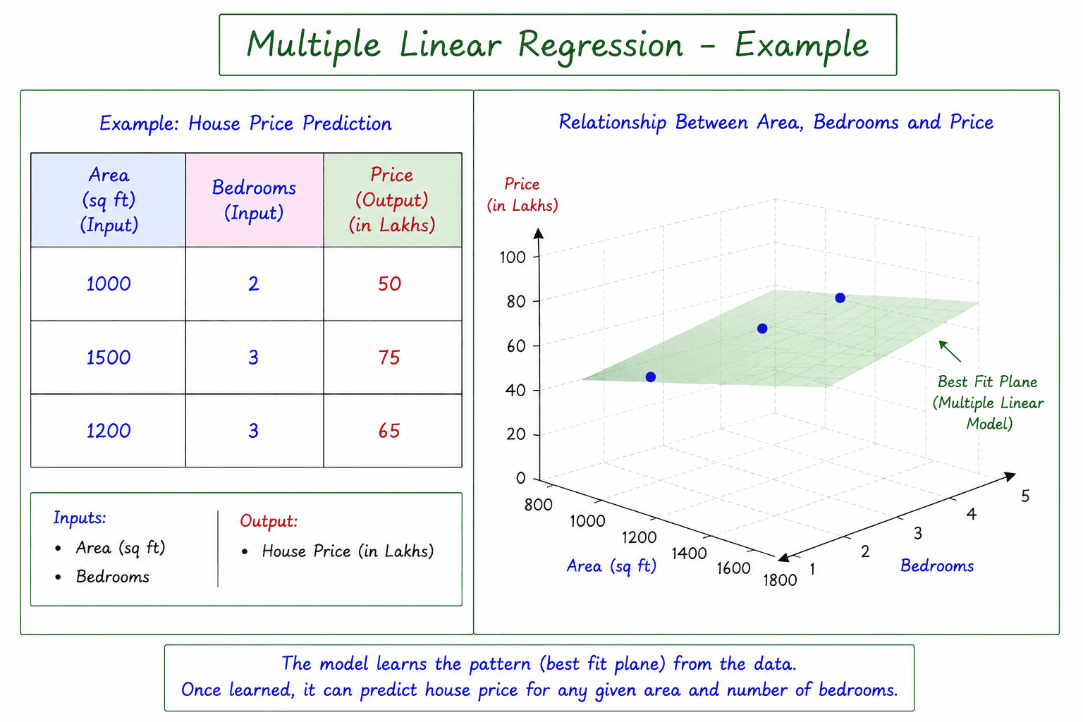
The diagram illustrates the relationship between Area, Number of Bedrooms, and House Price. Generally, larger houses with more bedrooms tend to have higher prices. Multiple Linear Regression learns this relationship from historical data and uses it to predict the price of new houses.
Multiple Linear Regression uses:
- Multiple input variables
- One output variable
Example
In the diagram:
Inputs (X₁, X₂) -> Output (Y)
Independent Variables (X₁, X₂) -> Dependent Variable (Y)
Area (sq ft), Number of Bedrooms -> House Price (Lakhs)
The table on the left contains historical data of houses showing their area, number of bedrooms, and selling price. The 3D graph on the right plots these values and illustrates the best-fit plane representing the relationship between the input variables and the house price.
Multiple Linear Regression Equation
The relationship between the inputs and output is represented by the equation:
\[y = b_0 + b_1x_1 + b_2x_2\]
Meaning of Terms
| Symbol | Meaning |
|---|---|
| y | Output or Target Variable |
| x1 | First Input / Feature (Area) |
| x2 | Second Input / Feature (Bedrooms) |
| b0 | Intercept |
| b1 | Coefficient of Area |
| b2 | Coefficient of Bedrooms |
Understanding the Equation
Suppose the model learns the following equation:
\[y=−5+0.04x1+12x2\]
where
- x1 = Area (sq ft)
- x2 = Number of Bedrooms
- y = House Price (Lakhs)
| Term | Meaning |
|---|---|
| Intercept = -5 | Estimated base price when all inputs are zero. |
| Coefficient of Area = 0.04 | Price increases by approximately 0.04 lakh for every additional square foot, keeping bedrooms constant. |
| Coefficient of Bedrooms = 12 | Price increases by approximately 12 lakhs for every additional bedroom, keeping area constant. |
Prediction Example
Using the learned equation
\[y=−5+0.04x1+12x2\]
Suppose a house has
- Area = 1400 sq ft
- Bedrooms = 3
Then
\[y=−5+0.04(1400)+12(3)\]
\[y=−5+56+36\]
\[y=87\]
Therefore, the predicted house price is
\[87 Lakhs\]
This predicted point can be visualized on the 3D graph where the Best-Fit Plane estimates the price corresponding to the given area and number of bedrooms.
Best-Fit Plane
Unlike Simple Linear Regression, which fits a straight line, Multiple Linear Regression fits a plane (or hyperplane when there are more than two input variables).
Many different planes can pass through the data points. However, Multiple Linear Regression selects the plane that minimizes the overall prediction error.
This plane is called the Best-Fit Plane.
- It passes as close as possible to the data points.
- It captures the relationship between multiple input variables and the output.
- It is used to predict unseen data.
In the graph shown in the diagram, the green surface represents the Best-Fit Plane, which models the relationship between area, bedrooms, and house price.
The goal of Multiple Linear Regression is to learn the relationship between multiple input variables and one output variable. Once this relationship is learned, the model can predict future values using the Best-Fit Plane.
3. Polynomial Regression
Polynomial Regression is a supervised machine learning algorithm used to predict a continuous numerical value. It models non-linear relationships between the input and output variables by fitting a curve instead of a straight line.
Although the relationship is non-linear, Polynomial Regression is still considered a type of Linear Regression because it is linear with respect to its coefficients.
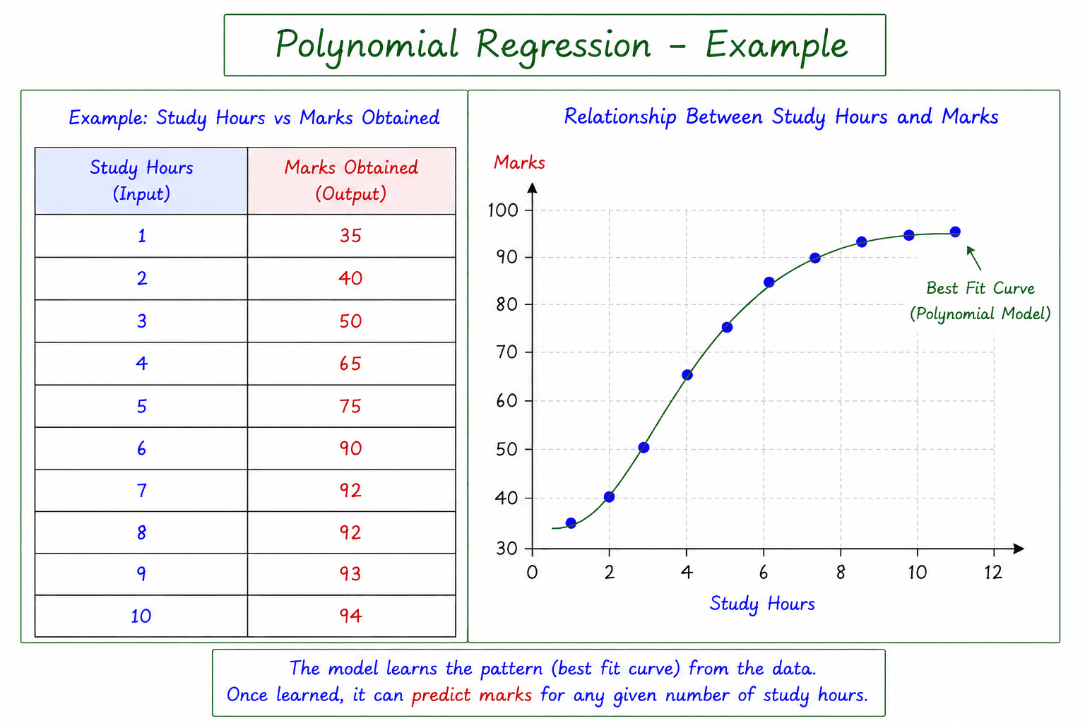
In the diagram:
Input (X) → Output (Y)
Study Hours → Marks Obtained
The table on the left contains historical data, while the graph on the right shows the data points and the Best-Fit Curve learned by the model.
Unlike Simple Linear Regression, which fits a straight line, Polynomial Regression fits a curve that better captures non-linear patterns in the data.
Common Polynomial Degrees
| Degree | Name | Equation | Typical Curve |
|---|---|---|---|
| 1 | Linear | \[y = a + bx\] | Straight Line |
| 2 | Quadratic | \[y = a + bx + cx^2\] | U-shaped Curve |
| 3 | Cubic | \[y = a + bx + cx^2 + dx^3\] | S-shaped Curve |
| 4 | Quartic | \[y = a + bx + cx^2 + dx^3 + ex^4\] | Multiple Bends |
| 5 | Quintic | \[y = a + bx + cx^2 + dx^3 + ex^4 + fx^5\] | More Complex Curve |